Insurance claims estimation and fraud detection with optimized deep learning techniques

Deep convolutional neural networks are targeted artificial neural networks specifically designed for image recognition tasks, which have been extraordinary achievements in this area. The term “deep” comes from the fact that there is a large number of layers, sometimes dozens or more stacked one on another in a DCNN architecture. Each layer has implemented filters to extract different features from the input image, and then these features are processed through non-linear activation functions that enable the network to learn sophisticated features in the data¹⁴.

DCNNs have been highly efficient in many related applications of image recognition, such as object detection, facial recognition, and medical image analysis. In addition, they found application in fraud detection tasks in various contexts. For instance, DCNNs are being used to identify fraudulent credit card transactions by learning patterns in transaction data that indicate such fraud. They also have been used to spot fraudulent insurance claims by analyzing images showing damage or injury and to distinguish between authentic and fake claims. In both of these cases, the foremost benefit of applying DCNNs for fraud detection is that they can automatically learn patterns indicative of fraud without requiring human feature engineering or any domain knowledge. This capability makes DCNNs a very effective weapon in fraud detection within vast and complex datasets.

Dataset description

The dataset used for training and evaluating the EHOA-CNN-12 model comprises 1,500 images from insurance claims, specifically designed for fraud detection in car damage assessments. These images are organized into the following classes:

• Headlamp Damage: 350 images.

• Door Dent: 400 images.

• Glass Shatter: 300 images.

• Tail Lamp Damage: 250 images.

• Unknown (Other): 200 images.

While the dataset is generally well-balanced, the “Unknown” class is slightly underrepresented. This reflects real-world fraud detection scenarios, where unidentified damage types are less common but still important to account for in the analysis.

To benchmark the performance of the proposed EHOA-CNN-12 model, a variety of models with differing architectures and depths were selected, including VGG16, VGG19, ResNet50, Custom CNN-12, and Custom CNN-15. These models were chosen based on their relevance to fraud detection in insurance claims and their capability to handle high-dimensional image data. Below is an overview of the reasoning behind the selection of each model:

• VGG16 and VGG19: VGG16 consists of 16 layers, while VGG19 includes 19 layers. Both models are widely used in image-based tasks due to their simplicity and depth. Utilizing small 3 × 3 convolutional filters, VGG models have demonstrated effectiveness in a variety of computer vision tasks, including fraud detection via image-based damage assessments. These models were selected to investigate how increasing depth affects the performance of fraud detection, particularly in recognizing complex patterns within image data.

• ResNet50: As a deep residual network, ResNet50 utilizes skip connections to mitigate vanishing gradients, enabling deeper networks to be trained more effectively. It has been proven successful in complex tasks with large, high-dimensional datasets. This model was chosen to evaluate the performance of deeper architectures with residual connections in comparison to the simpler VGG and custom CNN models, especially in the context of fraud detection.

• Custom CNN-12 and Custom CNN-15: These custom models, with 12 and 15 layers respectively, were designed to test simpler, less computationally intensive architectures. The inclusion of these models allows for experimentation with lower complexity architectures while still addressing fraud detection in insurance claims. Their purpose is to assess the trade-off between model complexity and computational efficiency, a critical consideration for real-world applications where both performance and efficiency must be balanced.

The comparison of these models facilitates a thorough evaluation of the EHOA-CNN-12 model by benchmarking it against a range of well-established architectures, each with varying levels of complexity and design principles. The following section discusses several of these models, including VGG16, VGG19, ResNet50, custom 12-layer, and custom 15-layer models, for insurance claims and fraud detection.

VGG16 deep learning model

The VGG16 model, which comprises 13 convolutional layers, 2 fully connected layers, and a SoftMax classifier¹⁵. The architecture of VGG16 is structured as follows:

• The number of feature kernel filters in each of the first and second convolutional layers is 64, all of which is 3 × 3 in size. These layers will process the input image, and the output result comes with dimensions of 224 × 224 × 64. The output of this then passes through a max pooling layer with a stride of 2.

• All the third and fourth convolutional layers have 128 feature kernel filters of size 3 × 3. After two max pooling layers with a stride of 2, which reduce the output size to 56 × 56 × 128.

• There are three blocks of convolutional layers, each with 256 feature maps, and a kernel size of 3 × 3.

• After these layers, there is a max pooling layer with a stride of 2.

• The eighth to thirteenth layers make up two blocks of convolutional layers. Each block contains 512 kernel filters of size 3 × 3, followed by a max pooling layer with a stride of 1.

• Fourteenth and fifteenth: These are fully connected hidden layers with 4096 units in each. The sixteenth is softmax output with 1000 units since classification is to be done.

Figure 1 depicts the VGG16 Model Architecture. The VGG16 model architecture is a deep network convolutional neural network that has been developed with an aim at image classification tasks. It comprises of 16 layers that include 13 convolutional layers, 3 fully connected layers, and 5 max-pooling layers. Convolution layers use small 3 × 3 filters with stride 1, whereas max-pooling layers use 2 × 2 filters with a stride of 2, progressively reducing spatial dimensions of the inputted image. The last layers are three fully connected layers. The last one outputs the class scores. VGG16 was known for its simplicity and depth. All of its convolutional layers were basically 3 × 3 filter sizes with same padding. The network could learn hierarchical features very efficiently. Though it is simple, the depth of VGG16 makes it capable of learning complex patterns in images, thus making it effective in most visual recognition tasks.

VGG19 deep learning model

In 2014, Simonyan and Zisserman introduced the VGG19 model, which contains 16 convolutional layers and 3 fully connected layers. This model will classify images in 1000 object categories as shown in Fig. 2. VGG19 is the one trained to extensive ImageNet database that contains a million images with 1000 different categories. This model gained prominence due to the distinctive utilization of multiple 3 × 3 filters in each convolutional layer. The architecture of VGG19 is composed of 16 convolutional layers for feature extraction, divided into 5 sets followed by max-pooling layers. This model takes the input as a 224 × 224-sized image and outputs the label for the object¹⁶.

ResNet50 deep learning model

The ResNet-50 architecture has 50 layers of neural networks and is designed with a stack of 3 layers. It is more accurate compared to the ResNet-34. The performance of the ResNet-50 model is 3.8 billion FLOP. The architectural diagram of ResNet-50 is shown in Fig. 3. There are 5 stages forming part of it, which includes a convolution block along with an identity block each. Every identity block contains 3 convolutional layers. ResNet contains skip connections which provide for addition at some points of the output of one layer to the output of another layer¹⁷.

ResNet-50 Architecture comprises different layers with specific functionalities. The layers in ResNet-50 are as follows: ni.\t Convolution layer: This layer features extraction from input images using filters to preserve pixel relations.ii.\tRectified Linear Unit (ReLU) layer: ReLU increases the nonlinearity in the input by providing an output value of zero for negative values and preserving positive values.

• Pooling layer: ResNet-50 applies max pooling to reduce the spatial dimensions of input, taking the maximum value from each of the 2 × 2 feature map elements with a stride of 2.

• The Flatten layer serves to convert the output from the previous layers, which could be multi-dimensional, into a 1D vector to feed it into the processing of the data.

• The Fully Connected layer takes in the output from the convolutional layers, which are rich in high-level features, and connects to fully connected layers.

• These layers enable learning nonlinear combinations of features, allowing the model in the end to capture complex patterns in the data.

• The Softmax function is the activation function in the final fully connected layer. It used for the purpose of predicting the probability of multiple classes in multiclass classification problems and helps make accurate and confident class predictions.

Custom CNN 12 layers

The customized CNN architecture is developed being simple and inspirational from others (Fig. 4) with popular CNN architectures such as VGG and LeNet. This architecture is sequential having 4 convolutional blocks and two fully connected layers. All the convolutional blocks apply the activation of Rectified Linear Unit (ReLU) to every convolutional layer, and there are a max pooling layer connected to the last convolutional layer. The first two blocks are called “Conv block 1” and contain 2 convolutional layers each; however, the last two blocks are called “Conv block 2” and contain 4 convolutional layers each¹⁸. The fully connected layers in this customized CNN architecture are of 64 nodes and 2 nodes, respectively. In the case of the last fully connected layer, softmax activation function is used for the prediction of probabilities about multiple classes in problems involving multiclass classification. The categorical entropy loss functions are used here, and optimization is done using Stochastic Gradient Descent. In a broad sense, this architecture is simple yet effective for many applications.

The custom CNN had 12 layers in their configuration and could, therefore function at multiple resolutions. It adopted a multi-stage architecture, favoring quick rejections of background regions in the early low-resolution stages, but then exhaustively examining a small set of candidates in the final high resolution stage. Localization effectiveness and the further reduction of candidate number are accomplished through a CNN-based calibration stage that is included after each detection stage of the architecture. The results demonstrate outstanding performance, with VGA-resolution images and a single CPU core to 14 FPS and, with the help of a GPU, as high as 100 FPS. This impressive efficiency, the custom CNN demonstrates the ability to effectively manipulate image data at various resolutions.

The EHOA-CNN-12 model creates a significant improvement to existing deep learning models for insurance fraud detection together with claims estimation despite not being an entirely new approach by handling optimization problems through effective local minimum resolution and slow convergence optimization. The integration between EHOA and custom CNN architecture produces enhanced model performance in addition to a demonstration of capabilities to optimize complex deep learning functionalities. The contributions made small progressive improvements which enhanced accuracy performance along with increasing efficiency and practical applicability in insurance fraud detection systems. The EHOA-CNN-12 model creates a significant improvement to existing deep learning models for insurance fraud detection together with claims estimation despite not being an entirely new approach by handling optimization problems through effective local minimum resolution and slow convergence optimization. The integration between EHOA and custom CNN architecture produces enhanced model performance in addition to a demonstration of capabilities to optimize complex deep learning functionalities. The contributions made small progressive improvements which enhanced accuracy performance along with increasing efficiency and practical applicability in insurance fraud detection systems. A straightforward architecture of the 12-layer CNN-Custom network can be seen in Fig. 5¹⁹. This shows the architecture and the structure or organization of the layers within the custom CNN.

Enhanced hippopotamus optimization algorithm (EHOA)

EHOA represents a novel optimization method based on hippopotamus movement that tackles two major problems facing deep learning models such as local minima traps and slow convergence. EHOA operates differently from standard optimization approaches since it implements automatic population size management and efficient solution space exploration. Enhanced performance from the algorithm stems from its precision in fine-tuning CNN model hyperparameters thereby accomplishing superior results than other advanced methods based on experimental validation. EHOA works as an integrated system with basic CNN architecture models to produce improved accuracy and operational efficiency together with robust performance necessary for actual fraud detection scenarios.

Optimizing hyperparameters is an important task for improving the accuracy and precision of the model. EHOA is utilized in the proposed method to optimize the hyperparameters of custom CNN model. The Enhanced Hippopotamus Optimization Algorithm (EHOA) is a novel optimization technique inspired by the social behavior of hippopotamuses. It addresses common challenges in traditional optimization algorithms, such as slow convergence and the tendency to become trapped in local minima, which are particularly evident in the original Hippopotamus Optimization Algorithm (HOA). Although HOA has shown potential in solving optimization problems, it is limited by inefficiencies in exploration and exploitation, as well as its static population size. In HOA, a population of candidate solutions was treated as hippopotamuses, and each individual, in search of an optimal solution, was to search the entire space in which it resides. The process of optimization moves these individuals through a fitness landscape in a way similar to hippopotamuses in search for food and each other. However, the basic HOA suffers from slow convergence and premature stagnation in very complicated landscapes of problems. EHOA addresses the shortcomings by introducing additional mechanisms such as adaptive and finer search strategy. These would be improved upon by adjusting the rates of exploration and exploitation based on the fitness of the individuals and the environment. The algorithm has a better position updating mechanism for the hippopotamuses ensuring that diversity in the search is maintained. The chances of falling into local optima are reduced, and EHOA thereby proves effective for solving complex, high-dimensional, and multi-modal optimization problems. EHOA introduces several key improvements over HOA:

• Dynamic Exploration-Exploitation Balance: In HOA, the exploration-exploitation balance is fixed, which can lead to suboptimal performance, especially in complex, high-dimensional spaces. EHOA improves upon this by dynamically adjusting the balance based on the fitness of individuals and the environment, enabling more effective search behavior. The exploration factor, denoted as , is dynamically adjusted as follows:

This dynamic adjustment ensures a more adaptable balance between exploring new areas of the search space and exploiting known good solutions.

• Adaptive Population Size: HOA uses a fixed population size, which can be inefficient when dealing with very large or small solution spaces. EHOA overcomes this limitation by introducing an adaptive population size, which allows the algorithm to adjust the population dynamically. This leads to better computational efficiency while maintaining high-quality solutions.

• Momentum-Based Updates: EHOA accelerates convergence by incorporating a momentum-based position update mechanism. Unlike HOA, where position updates are based solely on fitness values, EHOA introduces a momentum term, which helps to speed up convergence and improve stability throughout the optimization process.

• Hybrid Fine-Tuning: Once promising solutions are identified, EHOA introduces a hybrid fine-tuning phase to refine those solutions. This phase helps the algorithm avoid being trapped in local optima and ensures that the final solution is of higher quality, particularly in complex, multi-modal landscapes.

These enhancements make EHOA a more robust and efficient optimization technique, offering significant improvements in solving complex optimization problems.

In Eq. (2), the position of hippopotamuses is updated using a balance between exploration and exploitation where \(\:{X}_{i}^{old}\) is the current position of the ith hippopotamus, \(\:{P}_{best}\) is the personal best solution of the ith hippopotamus,\(\:\:{G}_{best}\) is the global best solution found so far, \(\:{\upalpha\:}\),\(\:\:{\upbeta\:}\) are the exploration and exploitation factors.

The fitness function in Eq. (3) determines the quality of the solution based on the problem at hand where \(\:\text{f}\left(\text{X}\right)\) represents the objective function for the optimization problem

In Eq. (1), an adaptive mechanism controls the balance between exploration and exploitation ensuring the effective search behavior where α is the exploration parameter and iteration is the current iteration of the algorithm.

In Eq. (4), a velocity is used to guide the movement of hippopotamuses in the search space to speed up convergence where \(\:{V}_{i}^{old}\) is the old velocity, w is the interia weight, c1,c2 are the learning factors, rand1,rand2 are random numbers in the range [0,1].

In Eq. (5), the algorithm stops when the convergence criteria are met such as maximum number of iterations o when the fitness improvement falls below a threshold where \(\:{Fitness}_{best}^{current}\) is the best fitness in the current iteration, \(\:{Fitness}_{best}^{previous}\) is the best fitness from the previous iteration and ϵ is small threshold value for convergence.

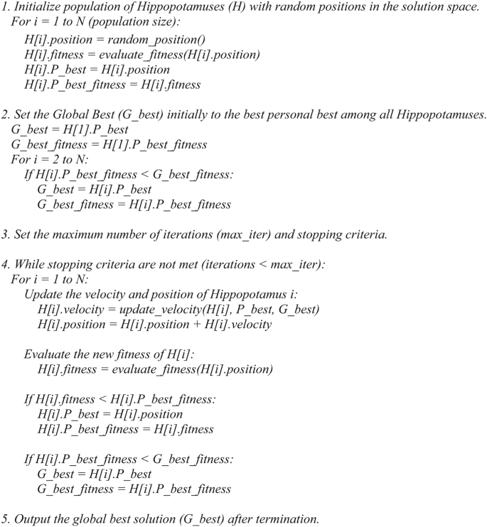
Figure 6 presents the iterative process of EHOA for optimization problems: Initial population of hippopotamuses with random position in the solution space. The fitness of each hippopotamus is calculated according to the objective function. The personal best (P_best) for each hippopotamus and the global best (G_best) across the entire hippopotamus population are determined. In subsequent generations, the updated positions of the hippopotamuses are determined by a mixture of their individual’s and global bests position, influenced by factors such as inertia factor and learning factor, and after assessing their fitness, the best solutions can be held. The process is continued until some stopping criteria that could be the maximum allowed number of iterations or convergence be met; the algorithm then outputs the global best as the optimized result. The algorithm of the proposed optimization algorithm is given below.

Comparison of HOA vs EHOA

The EHOA algorithm introduces several key enhancements over the original HOA, particularly in computational efficiency and performance. While HOA is often hindered by slow convergence and premature stagnation, EHOA effectively addresses these issues through dynamic adjustments to the exploration-exploitation balance, adaptive population size, and momentum-based updates. These modifications enable EHOA to converge more quickly and avoid getting trapped in local minima, making it particularly suitable for high-dimensional optimization problems.

• Computational Efficiency: EHOA is more computationally efficient than HOA due to its dynamic population size and momentum-based updates. HOA’s fixed population size can lead to inefficiencies, particularly in larger solution spaces. EHOA, on the other hand, optimizes the population size during the optimization process, reducing unnecessary computation once the solution space has been adequately explored.

• Performance: EHOA consistently outperforms HOA in terms of both accuracy and convergence speed. The adaptive exploration-exploitation balance and the hybrid fine-tuning phase contribute to improved solution quality, particularly in tackling complex, multi-modal, and high-dimensional optimization problems.

These advancements make EHOA a more robust and efficient optimization technique compared to HOA, especially when solving challenging optimization tasks.

Selection of hyperparameters

The selection of hyperparameters for both the CNN architecture and the Enhanced Hippopotamus Optimization Algorithm (EHOA) was informed by experimental trials as well as insights from existing literature. These hyperparameters were chosen with the aim of optimizing model performance and were further refined through the EHOA optimization process. The list of hyperparameters optimized by EHOA is detailed in Table 2.

Optimization process

• Iterations: The optimization process was run for 50 iterations, allowing for a comprehensive exploration of the search space and the fine-tuning of the model’s hyper parameters.

• Dynamic Exploration and Exploitation: During the optimization, the balance between exploration and exploitation was dynamically adjusted. This approach ensured that the algorithm could efficiently search for new solutions while also focusing on exploiting promising areas of the solution space.

• Final Hyperparameter Selection: After 50 iterations, the final hyperparameters were selected based on their performance on the validation set, ensuring the model achieved optimal performance.

Custom CNN 15 layers

The custom CNN architecture is composed of the layers Conv, pooling, and Fully Connected (FC), culminating in a softmax classification layer for generating class probabilities. This design capitalizes on sparse representation and parameter sharing to outperform logistic regression, Extreme Learning (EL), and Support Vector Machine (SVM) in terms of performance.

In Table 1, kernel sizes and node numbers for the extraction of local features like fruits or vegetables are deployed in a convolution operation. The outputs of the convolutional nodes are then put through an application of the ReLU function as a threshold to produce filtered features, which is the layer’s output. Pooling operations are used to generate the neighboring statistical summaries of such features and result in the creation of invariant representations. With ReLU as the activation function throughout the hidden layers, the model is trained with cross-entropy loss based on weighted training samples²⁰.

In the custom CNN architecture, a total of 15 layers exist, and the model was trained over 25 epochs; for the purpose of the results, the number of epochs that gave the best output is included. The FC layer would then multiply the input by a weight matrix and add a bias vector. The softmax layer utilized a softmax function that extended logistic regression for use in multiclass classification. By considering the class prior probability P(r) and the conditional probability of a sample given class r, P(x | r), the softmax layer calculates the class probabilities.

Then it can conclude that the probability of sample x belonging to class r is (6):

Here R is the total number of classes. If it define A_r as (7 & 8):

Then

The CNN model training algorithm applied to this paper was Stochastic Gradient Descent with Momentum (SGDM). This term stochastic means that the mini-batch training method is applied, with a batch size of 128. The learning rate was initialized to 0.01 and reduced by a factor of 10 every 10 epochs, and a momentum of 0.9 was set to assist in optimization. The maximum number of epochs was set to 30. This determines when the training process would stop. In this case, since it is a multiclass problem, cross entropy is selected as the loss function.

Computational requirements of the proposed model

The EHOA-CNN-12 model integrates the Enhanced Hippopotamus Optimization Algorithm (EHOA) for hyperparameter optimization, which introduces additional computational overhead compared to traditional CNN architectures. However, the efficiency of the EHOA in dynamically adjusting the exploration-exploitation balance and fine-tuning hyperparameters leads to enhanced model performance, justifying the extra computational cost.

To assess the computational efficiency and scalability of the EHOA-CNN-12 model, an analysis of training time and resource usage was conducted. The experiment was performed on a system with the following specifications:

These specifications allowed for an in-depth evaluation of the model’s computational demands and its ability to scale during training. Despite the added computational cost of the EHOA, the model demonstrated improved performance, which validated the trade-off between efficiency and resource usage.