
This study was conducted as a single-center study. This retrospective observational study was conducted in accordance with the 1989 Helsinki Declaration and was approved by the Non-Interventional Clinical Research Ethics Committee of Erzincan Binali Yıldırım University Faculty of Medicine. All methods used in this study were performed in accordance with the relevant guidelines and regulations. All patient records who were diagnosed with Pulmonary Embolism and treated at İzmir Atatürk Training and Research Hospital between 2016 and 2020 and were over the age of 18 were retrospectively reviewed. No sampling method was used for the number of data. All patients who met our criteria during the specified period were included in the study. The characteristics of the patients examined were analyzed and twenty variables without missing data were determined (Table 1). The age, gender and accompanying diseases of these patients were also recorded.
Characteristics of participants, inclusion and exclusion criteria, defining workflow and datasets
The patient cohort of this study consisted of patients diagnosed by contrast-enhanced multidetector computed tomography (CT) with echocardiography and lower extremity venous Doppler ultrasound reports. We excluded pregnant patients, those for whom echocardiography and Doppler ultrasound reports were not available, individuals with chronic thromboembolic pulmonary hypertension, and those with known right heart dysfunction. Patients younger than 18 years were excluded. A total of 163 patients, 80 (49.1%) females and 83 (50.9%) males, were included in the study. RVD was observed in 27 patients (16%).
Standard transthoracic echocardiography was performed in all patients on admission, preferably within 48 h of diagnosis. Thrombus location was determined according to official radiology reports. Echocardiography and lower extremity venous Doppler ultrasonography reports were analyzed for right ventricular dysfunction and deep vein thrombosis. Right ventricular enlargement was defined as baseline RV diameter greater than baseline LV diameter or baseline and mid-RV diameters > 41 mm and > 35 mm, respectively. We used the following criteria to diagnose right ventricular dysfunction: Tricuspid annular plane systolic excursion (TAPSE) < 16 mm, Tricuspid Lateral Annular Systolic Velocity < 9. Doppler tissue imaging showed a 5 cm/sec, flattened interventricular septum in parasternal short axis view, dilated inferior vena cava, decreased inspiratory collapse in subcostal view, pulmonary ejection acceleration time < 60 msec, and peak systolic gradient between the mid-systolic notch and the right ventricle and right atrium < 60 mmHg (10, 11).
The 20 characteristics of the dataset (see Supplementary Materials) of patients diagnosed with PE in this study are given in Table 1. RVD diagnosis was coded as 1: Presence, 0: Absence. The database contains a total of 163 vectors distributed into two classes, Class_1 (0: Absence) and Class_2 (1: Presence). Class_1 contains 136 elements and Class_2 contains 27 elements. The class data is unbalanced as there is a large difference between the number of elements of class 1 and the number of elements of class 2. In such cases, the classification accuracy (ACC) metric does not make much sense. Therefore, we use MCC metric for classification accuracy (see Sect.”ML models”).
Feature 2 (Age) is presented in the form of discrete values in the range of 22–93 years; feature 12 (Appearance of DVT) has 3 gradations; the remaining features are presented in binary form. The RVD examination result was also presented in binary format (1: Presence, 0: Absence). DVT: Deep vein thrombosis.
ML models
Architecture of LogNNet feature selection method and hyperparameter optimization
LogNNet is a neural network based on the technology of “reservoir calculation with automatic generation of weight coefficients”. The structure of the LogNNet neural network is summarized in Fig. 1. The work had three main stages: data collection, LogNNet training with the selection of main features, and testing of feature combinations. The process begins with feeding Pulmonary Embolism patient data into the neural network. These data undergo a structured transformation and training process, which can be divided into the following detailed steps:
-
1.
Input Dataset: The dataset includes key features for diagnosing or predicting pulmonary embolism, essential for training the neural network.
-
2.
Normalization: The input vector Y (dimension d) is normalized to ensure all data falls within a standard range, facilitating model learning by reducing data scale biases.
-
3.
Matrix Reservoir: A reservoir matrix W with n rows serves as the core of the LogNNet network, capturing dynamic data crucial for learning.
-
4.
Chaotic Series Filling: The reservoir is filled with chaotic time series X, introducing complexity and aiding the network in adapting to varied data forms.
-
5.
Multiplication Process: The product S is generated by multiplying W by Y, creating a rich input representation by combining chaotic dynamics with normalized data.
-
6.
Normalized Vector: The product S is further normalized to Sh, ensuring consistent data before input to the classifier.
-
7.
Output Classifier: The classifier interprets the normalized vector Sh to produce predictions, essential for analyzing the transformed data.
-
8.
Training Stage: The model adjusts parameters using labeled data, learning to recognize chaotic patterns and classify or predict accurately.
-
9.
Testing Stage: Performance is evaluated with unseen data, confirming the neural network’s accuracy and generalizability for pulmonary embolism data.

The workflow of the work and the main stages of calculation. This figure summarizes the main stages of the study for the diagnosis of RVD in patients using data from Pulmonary Embolism patients (https://data.mendeley.com/datasets/bm4v4rzdyd/1). These stages are: data collection, training LogNNet with the selection of main features, testing the combinations of the most important features affecting the diagnosis of the disease. The image in the upper left section represents the demographic characteristics and clinical findings of PE patients. The patient’s “Gender” is represented by male and female icons; the patient’s “Age” is between “16 and 90”; “Coronary Artery Disease” and “Thrombus Segment” and other features represent the patient’s clinical findings. The upper right image was generated by the Chat GPT (version 4.0) artificial intelligence program. The upper right image represents a conceptual clinical environment in which the characteristics of PE patients can be observed. No real patient data or personally identifiable information was used, ensuring that ethical standards were followed. The lower image shows the general architecture of LogNNet, shows the training and testing process. The upper left and lower left images were created by the authors.
The LogNNet parameters in the software implementation were set as follows. LogNNet_params = {‘num_rows_W’: (2, 100), ‘limit_hidden_layers’: ((1, 60), (1, 60), (1, 60)), ‘learning_rate_init’: (0.001, 0.1), ‘n_epochs’: (4, 800), ‘n_f’: −1, ‘selected_metric’: ‘mcc’, ‘num_folds’: 100, ‘tol’: 1e-7,}
The parameter ‘num_rows_W’ defines the number of rows in the reservoir W, formed from the chaotic time series X, whose length depends on the length of the input vector Y and the number of rows in the reservoir. This parameter is selected using the PSO (Particle Swarm Optimization) method within the range of 2 to 100. The parameter ‘limit_hidden_layers’ is also optimized using PSO and defines the number and sizes of hidden layers; for example, ((1, 60), (1, 60), (1, 60)) denotes three hidden layers, each with limits from 1 to 60 neurons. This format allows flexible control over the number of layers by adding new limits to the configuration. The parameter ‘learning_rate_init’ determines the initial learning rate of the optimizer: a rate that is too high leads to model instability, while a rate that is too low slows down the training. The PSO method is also used to select ‘n_epochs’ (the number of epochs) and ‘tol’ (tolerance), the stopping criterion for training.
The LogNNet model was evaluated using the all metric, specified by the parameter ‘selected_metric’. The parameter ‘num_folds’ specifies the number of repeated stratified calculations, with the process repeated 100 times.
The parameter ‘n_f’ defines the feature selection in the input vector; it can be a list of indices (e.g1,2,7), a range (e.g., (2, 5)), or a number indicating the total number of features used, where PSO selects the best combination. A value of n_f = ‘−1’ allows all features to be used.
To implement an ensemble model consisting of 500 individual LogNNet models, the following procedure was applied:
-
1.
A dataset was generated containing the selected features and the target column.
-
2.
Five base models were initialized, each with unique reservoir configurations tailored to their respective feature sets. The relatively small number of base models was chosen due to the computational cost—each full training cycle requires approximately 7 min. Notably, the reservoir optimization was performed with the num_folds parameter set to 100, which ensures robust tuning of the chaotic reservoir even on small datasets.
-
3.
In a loop of up to 500 iterations, these five base models sequentially updated their output (MLP) layers using 80% of the dataset by applying the model.fit_MLP function (see documentation for details50 and Sect.”Classification Metrics Calculated with Repeated Stratified Hold-out Approach, Ensemble Method”.). This fine-tuning step is computationally inexpensive, taking only milliseconds per model.
As a result, an ensemble of 500 unique LogNNet models was obtained.
The calculations were conducted using the LogNNet package version 1.650.
Other machine learning methods
Common machine learning methods were used for comparison with the above classification methods: random forest (RF)51 and support vector machine (SVM)52. Every machine learning model was a pipeline consisting of three successive stages: imputation, numerical processing of non-discrete features and classification (RF or SVM). All ML models was implemented using scikit-learn library53.
The imputation of missing feature values was done using the most frequent value of this feature. Since the presented dataset contains missing values only in discrete features, this method seems to be the most suitable. To reduce the influence of outliers in the non-discrete feature (Age), the method of numerical transformation (robust scaling) was used. Scaling the feature value was carried out by subtracting the median and scaling the data according to the quantile range.
The selection of optimal hyperparameter’s values of the classifiers was carried out based on the MCC value (Sect.”Classification Metrics Calculated with Repeated Stratified Hold-out Approach, Ensemble Method”).
Classification metrics calculated with repeated stratified Hold-out approach, ensemble method
The primary evaluation metric chosen for this study was MCC41, specifically due to its effectiveness in handling imbalanced datasets, such as ours, by measuring the correlation between observed and predicted classifications. MCC is especially useful in medical contexts as it considers the balance across all classes, providing a robust assessment of model performance.
Additional metrics were used to gain a more comprehensive understanding of model effectiveness: Accuracy, Sensitivity, Specificity, Precision, F1 Score.
Accuracy measures the model’s overall ability to correctly classify cases. However, in scenarios with class imbalance (such as a higher prevalence of healthy cases), accuracy alone may not fully reflect model performance, making it essential to interpret in conjunction with other metrics.
Sensitivity, or recall, quantifies the model’s capacity to correctly identify positive cases (e.g., diseased individuals). This metric is particularly critical in clinical settings where the ability to detect true positives is essential to avoid missing critical cases.
Specificity assesses the model’s accuracy in identifying negative cases (e.g., healthy individuals). High specificity is important for minimizing false positives, which is valuable in reducing unnecessary treatments and preventing overtreatment of healthy patients.
Precision indicates the accuracy of the model’s positive predictions by showing the proportion of true positives among predicted positives. Higher precision helps reduce the burden of unnecessary follow-up testing by ensuring that positive predictions are more likely to be correct.
The F1 score combines sensitivity and precision, providing a balanced measure of the model’s ability to both detect and accurately classify positive cases. This score is valuable for evaluating models where both sensitivity and precision are important, ensuring critical cases are effectively managed without excessive false positives.
Due to the limited size of our dataset, we could not afford the traditional procedure of splitting the dataset into fixed training and independent test sets for ensemble evaluation. Instead, we employed a repeated stratified hold-out procedure54 (500 iterations) for training individual ML models. Each iteration involved an independent random stratified split (80% training, 20% testing), allowing comprehensive coverage and robust estimation of model performance. While each individual model was tested separately, we recognize that, in practice, the ensemble of all 500 models with majority voting will likely outperform the average performance of a single model due to variance reduction. Thus, the metrics obtained from our repeated stratified hold-out approach should be interpreted as a conservative upper-bound estimate of the ensemble’s performance. The actual performance of the practically deployed ensemble model is expected to be equal or superior to this estimate.
We empirically explored ensemble sizes ranging from 10 to 1000 models and observed that after approximately 500 models, the confidence interval of the Matthews correlation coefficient (MCC) for the main feature combinations decreased to below 1% of its mean value. This indicated that further increasing the number of models yielded negligible improvements in predictive stability. Therefore, an ensemble size of 500 models was selected as an optimal compromise between result reliability and computational efficiency.
Figure 2 presents a flowchart illustrating the algorithm’s workflow, from data preprocessing to the final ensemble prediction.
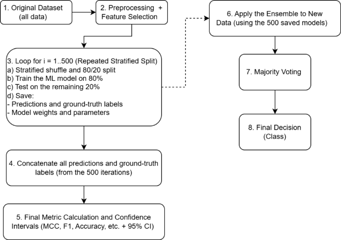
Example flowchart illustrating the repeated stratified hold-out procedure (Steps 1–5) combined with the ensemble methodology (Steps 6–8).
Step 1. Original Dataset: The complete initial set of data samples.
Step 2. Preprocessing and Feature Selection: Removal of missing values, data normalization, and selection of informative features, among other preprocessing steps.
Step 3. Repeated Stratified Hold-Out Procedure (i = 1 to 500):
-
a.
Each iteration employs an independent random stratified hold-out split, maintaining class proportions (80% training, 20% testing).
-
b.
A separate ML model is trained using the training subset (80%).
-
c.
Testing: The trained model generates predictions on the independent testing subset (20%).
-
d.
Saved items: (1) predicted labels and corresponding true labels for later aggregation, and (2) trained model parameters (weights and hyperparameters).
Step 4. Concatenation of Results: All predictions and true labels from the 500 iterations are aggregated into unified arrays.
Step 5. Final Metric Calculation: Performance metrics (MCC, Accuracy, F1-score, etc.) and associated confidence intervals (e.g., via percentiles or bootstrap) are calculated from these aggregated arrays.
Step 6. Ensemble Application: For classifying new data in practice, predictions are obtained using all 500 previously trained models.
Step 7. Majority Voting: Each of the 500 classifiers generates an individual prediction, and the final class assignment is determined through majority voting.
Step 8. Final Decision: The ensemble outputs the final predicted class for the new data sample.
The presented flowchart thus highlights:
-
The repeated stratified hold-out procedure for robust model evaluation (500 iterations),
-
Mechanisms for aggregating results to reliably estimate performance metrics, and.
-
Subsequent practical deployment of the ensemble model with majority voting for classifying new data.
To estimate the 95% confidence interval (CI) for the final MCC value we performed the cross-validation procedure N = 100 times. The resulting metric values were used to calculate the standard error and then CI.
The calculations were performed on a personal computer with an AMD Ryzen 9 3950X processor and 64 GB of DDR4 RAM.
The software environment consisted of Python 3.8, and we used the NumPy and scikit-learn libraries for data processing and modeling.
Threshold approach for a single feature
The single feature threshold approach uses a simple model with a single clinical threshold, Vth, that separates two classes. This threshold can be seen as an analog to a clinical decision threshold, commonly used in medical diagnostics. In this model, there are two types of predictors: positive predictors, which correlate with the presence of the condition when the feature exceeds Vth, and negative predictors, which indicate the absence of the condition under similar conditions.
$$\left\{ \begin{gathered} {\text{Positive predictor: if feature value > }}{V_{th}}{\text{ }} \hfill \\ {\text{ then RVD (1: Presence) }} \hfill \\ {\text{ else RVD (0: Absence) }} \hfill \\ {\text{Negative predictor: if feature value > }}{V_{th}}{\text{ }} \hfill \\ {\text{ then RVD (0: Absence) }} \hfill \\ {\text{ else RVD (1: Presence)}} \hfill \\ \end{gathered} \right.$$
(1)
For binary features, it convenient to represent positive and negative predictors in a truth table format.
$$\left\{ \begin{gathered} {\text{Positive predictor: }}\begin{array}{*{20}{c}} {{\text{feature value}}}&\vline & {{\text{RVD}}} \\ 0&\vline & {{\text{0: Absence}}} \\ 1&\vline & {{\text{1: Presence}}} \end{array}{\text{ }} \hfill \\ {\text{Negative predictor: }}\begin{array}{*{20}{c}} {{\text{feature value}}}&\vline & {{\text{RVD}}} \\ 0&\vline & {{\text{1: Presence}}} \\ 1&\vline & {{\text{0: Absence}}} \end{array} \hfill \\ \end{gathered} \right.$$
(2)
Synergy effect metric
To evaluate the synergistic contribution of using N features compared to a single feature, the characteristic synergistic effect coefficient Ksyn was employed. The synergistic effect coefficient Ksyn was estimated using the following formula:
$$K_{syn} = \frac{1- max(MCC[Feature \:1], MCC[Feature \: 2],\ldots ,MCC[Feature \: N])}{1.001-MCC[Feature\:1, Feature\:2,\ldots,Feature\:N]}\:,$$
(3)
where:
-
Max denotes the maximum value selection function,
-
MCC[Feature] represents the MCC value calculated using each individual feature,
-
MCC[Feature 1, Feature 2,…,Feature N] represents the MCC value calculated using the combination of N features.
This coefficient Ksyn allows us to assess the degree of synergistic improvement when combining multiple features, highlighting whether the joint contribution of features enhances the predictive performance beyond what is achievable with the best single feature alone.


