How Roblox uses machine learning-optimized bloom filters to reduce the cost of Spark join queries

abstract

70 on Roblox every day 1 million users participating in millions of experiences, totaling 16 1 billion hours per quarter. This interaction produces petabyte-scale data lakes powered for analytics and machine learning (ML) purposes. Joining fact and dimension tables in a data lake is resource-intensive, so we employed a trained Bloom filter to optimize this and reduce data shuffling. [1]- Smart data structures using ML. These filters significantly trim the combined data by predicting their presence, increasing efficiency and reducing costs. Along the way, we also improved the model architecture and demonstrated significant benefits in reduced memory and CPU processing time, and improved operational stability.

introduction

In a data lake, fact tables and data cubes are temporarily partitioned for efficient access, but dimension tables have no such partitions, and joining them with the fact table during updates is resource-intensive. The key space of a join is determined by the temporary partition of the fact table being joined. The dimensional entities that exist in that time partition are a small subset of the dimensional entities that exist in the entire dimensional dataset. As a result, most of the shuffled dimension data in these joins is eventually discarded.. To optimize this process and reduce unnecessary shuffling, I considered using the following: bloom filter We were using separate join keys, but were running into problems with filter size and memory footprint.

To address them, we investigated Trained bloom filteris an ML-based solution that reduces the size of Bloom filters while keeping the false positive rate low. This innovation improves the efficiency of join operations by reducing computational costs and increasing system stability. The following diagram illustrates the traditional optimized join process in a distributed computing environment.

Improving combination efficiency with trained Bloom filters

We employed a learned Bloom filter implementation to optimize the joins between fact and dimension tables. We built an index from the keys present in the fact table and then deployed that index to pre-filter the dimensional data before the join operation.

Evolution from traditional Bloom filter to learned Bloom filter

Traditional Bloom filters are efficient, but add 15-25% additional memory per worker node that must be loaded to reach the desired false positive rate. However, by using Learned Bloom Filters, we were able to significantly reduce the index size while maintaining the same false positive rate. This is because Bloom filters are transformed into binary classification problems. A positive label indicates that the value is present at the index, and a negative label means that the value is not present.

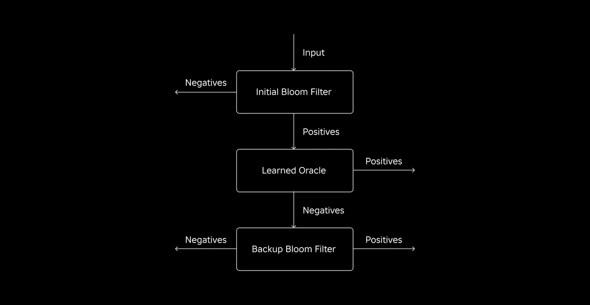
The introduction of an ML model facilitates an initial check of the values, followed by a backup Bloom filter to eliminate false negatives. The reduction in size is due to the compressed representation of the model and the reduction in the number of keys required for the backup Bloom filter. This differs from the traditional Bloom filter approach.

As part of this work, we established two metrics to evaluate the trained Bloom filter approach: the final serialized object size of the index and the CPU consumption when executing join queries.

Overcoming implementation challenges

Our first challenge was to deal with a highly skewed training dataset with few dimension table keys in the fact table. We observed that approximately one-third of the keys were duplicated between tables. To address this, we utilized a sandwich learning Bloom filter approach. [2]. It integrates the earlier traditional Bloom filter and rebalances the dataset by removing most of the keys that were missing from the fact table, effectively eliminating negative samples from the dataset. Then, only the keys included in the first Bloom filter, along with any false positives, were transferred to an ML model called the “learned oracle.” This approach resulted in a balanced training dataset for the learned oracles and effectively overcome the bias issue.

The second challenge focused on the model architecture and training capabilities. This is different from the classic problem of phishing URLs. [1]the join key (in most cases a unique identifier for the user/experience) was not inherently informative. This led us to investigate dimensional attributes as a potential model feature to help predict whether a dimensional entity is present in a fact table. For example, imagine a fact table containing user session information about experiences in a particular language. The geographic location or language preference attributes in the User dimension are good indicators of whether an individual user is present in the fact table.

For the third challenge, inference delay, we needed a model that minimized false negatives and provided a fast response. For these key metrics, the gradient-boosted tree model is the best choice, and we have reduced its feature set to balance accuracy and speed.

Here is the updated join query with the learned Bloom filter:

result

Here are the results of an experiment using Bloom filters trained on a data lake. We consolidated these into five production workloads, each with different data characteristics. The most computationally expensive part of these workloads is the join between fact and dimension tables. The fact table key space is approximately 30% of the dimension table. First, we discuss how the trained Bloom filter outperformed the traditional Bloom filter in terms of final serialized object size. Next, we demonstrate the performance improvements observed by integrating Learned Bloom Filters into the workload processing pipeline.

Size comparison of trained Bloom filters

As shown below, when looking at specific false positive rates, the two learned Bloom filter variants improve the total object size by 17-42% compared to the traditional Bloom filter.

Furthermore, by using a smaller subset of features in the gradient-boosted tree-based model, we were able to speed up inference while minimizing optimization losses by a fraction.

Results of using the learned Bloom filter

In this section, we compare the performance of Bloom filter-based joins to that of regular joins across several metrics.

The following table compares the performance of workloads with and without trained Bloom filters. A trained Bloom filter with a total false positive probability of 1% shows the following comparison while maintaining the same cluster configuration for both join types.

First, we found that the Bloom filter implementation performed 60% better than regular joins in CPU time. The additional compute spent evaluating the Bloom filter increased the CPU usage of the scan step of the trained Bloom filter approach. However, the pre-filtering done in this step reduced the size of the shuffled data, reducing the CPU used in downstream steps and reducing the total CPU time.

Second, the trained Bloom filter has about 80% less total data size and writes about 80% fewer total shuffle bytes than a regular join. This makes join performance more stable, as explained below.

Reductions in resource usage were also observed for other production workloads during the experiment. Average values were generated by the learned Bloom filter approach over a two-week period across all five workloads. Everyday cost reduction of twenty five%,This also includes training and indexing the model.

By reducing the amount of data that is shuffled while performing joins, we were able to significantly reduce the operating costs of our analytic pipeline, while increasing the stability of our analytic pipeline. The following graph shows the variation (using the coefficient of variation) in the execution duration (measured time) for the regular join workload and the trained bloom filter-based workload over a two-week period for the five workloads we experimented with. Executions using trained Bloom filters are more stable and more consistent in duration, opening the possibility of moving to cheaper, temporary, and less reliable computing resources.

References

[1] T. Kraska, A. Beutel, EH Qi, J. Dean, and N. Polyzotis. For learned index structures. https://arxiv.org/abs/1712.012082017.
[2] M. Mitzenmacher. Optimizing trained bloom filters by sandwiching.
https://arxiv.org/abs/1803.014742018.
¹As of 3 months ending June 30, 2023
²As of the three months ended June 30, 2023