Flood susceptibility assessment using three machine learning techniques and comparison of their performance

Study area

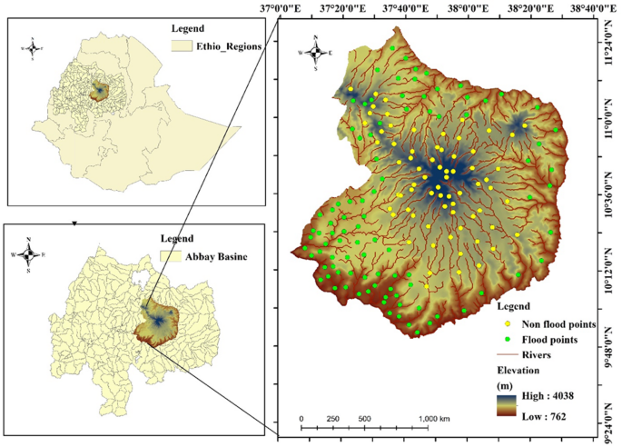
Choke is a large block of the highland mountain range, located in the central part of both the East and West Gojjam Administrative Zones in the Amhara National Regional State, northwestern Ethiopia. Choke Mountain serves as a water tower for the upper Blue Nile Basin, acting as the source for over 60 rivers and 270 springs³⁸. The catchment area of Choke Mountain spans nine woredas, and the watershed is situated between 9° to 11°N latitude and 37° to 38°E longitude (Fig. 1). Diverse topographical features, ranging from plateaus and deep incised valleys to escarpments, plains, and gorges, characterize the region. Elevations within the area vary from 2,800 to 4,088 m above sea level. Due to the complexity of its topography, the region experiences significant local gradients in precipitation, temperature, and soil properties³⁹. Choke Mountain is pivotal to the region’s hydrology, being the primary source of the majority of the tributaries of the Blue Nile River. Among the four major rivers originating from the mountain are the Muga, Chemoga, Abeya, and Techma, in addition to several smaller tributaries (Abay)³⁹. The mountain’s abundant water resources support various nature-based tourism activities, including swimming, boating, hiking, and fishing. These water resources are also crucial for other purposes, such as electricity generation, drinking water, irrigation, and washing. Climatically, the Choke Mountain region spans six distinct climatic zones: Upper Kola, Lower Weyna Dega, Upper Weyna Dega, Lower Dega, Upper Dega, and Wurch⁴⁰. Rainfall in the region is highly variable, ranging from 600 to 2,000 mm per year, with local differences due to the topographic gradients⁴¹. The dominant soil types in the watersheds include Leptosols, Cambisols, Vertisols, Nitosols, Alisols, Luvisols, Andosols, and Phaozems, which support a variety of agricultural activities. Common crops cultivated in the region include sorghum, maize, teff, durum wheat, barley, chickpeas, and various pulses and potatoes, depending on the agro-ecological zone⁴². Maps were created using ArcGIS software (version 10.4; Esri, Redlands, CA, USA; https://www.esri.com).

Major flood incidents during the last ten years were compiled from the National Disaster Risk Management Commission (NDRMC), the National Meteorological Agency (NMA), existing research, and remote sensing assessments to put the significance of flood susceptibility assessment into perspective (Table 1). Recurrent flooding in the Choke Watershed has caused agricultural losses, displacement, and infrastructural damage throughout the Kiremt (major rainy) season, which runs from June to September. This recurrent trend emphasizes the necessity of data-driven mapping of the region’s flood susceptibility.

Flood inventory map

Flood susceptibility mapping is a binary classification process that assigns a value of 1 to flood-affected locations and 0 to non-flood-affected locations^4,45. In this study, a flood inventory map was developed to represent spatially distributed flood and non-flood areas based on five significant flood events that occurred in 2005, 2010, 2013, 2016, and 2020. Data were primarily obtained from the National Disaster Risk Management Commission (NDRMC), Sentinel-1 Synthetic Aperture Radar (SAR) imagery, and complementary hydrological and logistical records^44,46,47.

For each flood event, pre- and post-flood Sentinel-1 SAR images were mosaicked and processed using speckle filtering to minimize image noise. The inundated areas were identified using a change detection analysis, and then flooded pixels were identified using a 1 (positive) value and non-flooded locations using a 0 (negative) value. This was done using threshold-based classification. To ensure precise delineation of flood extents, a Digital Elevation Model (DEM) was utilized to rectify geometric distortions and eliminate permanent water bodies and high slopes (> 5%)^4,26.

Ultimately, a total of 300 observation points were identified for the flood inventory map, comprising 210 flood-affected and 90 non-flood-affected locations. To improve dataset representativeness and reduce potential class imbalance, an additional 120 non-flood points were randomly generated in well-drained, flood-free areas, resulting in a balanced dataset of 210 flood and 210 non-flood points for modeling.

The non-flood points were carefully selected from higher elevation, well-drained, and flood-free areas confirmed through DEM-derived slope and elevation data. Their reliability was validated using multi-temporal analysis of Sentinel-1 SAR imagery, Google Earth Pro time-series inspection, and field verification during dry seasons. Additionally, historical flood records (2000–2020) and flood damage reports were reviewed to confirm the absence of inundation. A buffer zone was created around previously flooded areas to avoid selecting non-flood points near transitional or potentially flood-prone zones. This combined approach ensured the credibility and spatial representativeness of the non-flood samples^26,45,48.

The dataset was divided into 70% for model training and 30% for validation, following established practices in flood susceptibility studies^29,49,50,51. This ratio provides an optimal balance between ensuring sufficient data for model training—enabling the algorithms to capture spatial variability and complex feature relationships—and maintaining a robust independent validation subset for performance assessment. Several previous flood-related studies have demonstrated that a 70:30 (or similar 75:25) ratio yields stable and generalizable model results while avoiding overfitting⁵². In this study, the chosen split ensured that the models were trained with an adequately large and diverse dataset while preserving enough data to independently validate predictive accuracy and generalization capability.

The methodological flowchart followed in this study is shown in Fig. 2.

Flood-influencing factors

Previous studies have identified four primary groups of factors influencing flood occurrence: geomorphological, geological, hydrological and climatic, and anthropogenic activities⁵³. Based on these studies and the availability of relevant data in the study area, eleven flood-conditioning factors were selected for analysis. These include elevation, slope, aspect, plan curvature, topographic wetness index (TWI), SPI, drainage density (Dd), distance from river, soil types, land use/land cover (LULC), and rainfall patterns.

Digital Elevation Model (DEM) data were obtained from the obtained from ALOS-PALSAR. From the DEM, key topographic parameters such as elevation, slope, aspect, plan curvature, Dd, and TWI were derived. These parameters are widely used in previous flood susceptibility studies due to their effectiveness in accurately mapping potential flood-prone areas. All spatial data were processed and resampled within a Geographic Information System (GIS) environment; using raster data with a spatial resolution of 30 m (see Table 2 for data sources).

Elevation

Elevation is a critical factor in flood risk modeling, as it directly influences the flow of water during flood events. Water generally follows the path of least resistance, typically along the steepest descent⁵⁴. In this study, elevation data were derived from the Digital Elevation Model (DEM) obtained from ALOS-PALSAR. It was downloaded from the Alaska Satellite Facility (ASF) website (https://www.asf.alaska.edu) at a spatial resolution of 12.5 m. This dataset was used to generate the elevation model of the Choke Mountain Watershed (Fig. 3a).

Using elevation data, identify flood-prone areas, estimate the extent and severity of potential flooding, and assess the likely impacts on infrastructure, communities, and ecosystems. Accurate elevation data are essential for developing effective flood risk management strategies. Thus, elevation is a fundamental parameter in flood susceptibility assessment⁵⁴. Low-lying or flat areas are generally more susceptible to flooding due to slower water drainage and accumulation. Understanding the region’s topography and related geomorphological features is therefore vital for assessing flood vulnerability. Areas at lower elevations tend to experience higher flood risk⁵⁵. Maps were created using ArcGIS software (version 10.4; Esri, Redlands, CA, USA; https://www.esri.com).

Slope

Slope is another key parameter in flood modeling, as it affects both the velocity and direction of surface water flow. Slope refers to the steepness or inclination of the terrain and is commonly derived from DEM data. Steeper slopes typically result in faster runoff and greater erosion potential, while flatter areas may experience slower drainage and increased water accumulation¹. However, flood risk is influenced by additional factors such as land use, vegetation cover, and soil characteristics⁵⁴. In some contexts, gentle slopes can extend the time available for infiltration, but they can also lead to a larger volume of surface runoff entering drainage systems, thereby increasing flood risk⁵⁴. In this study, a slope map was generated using ArcGIS 10.4 software https://www.esri.com) from the DEM. The slope data were then classified into five categories to facilitate flood risk analysis (Fig. 3b).

Aspect

Aspect is a key factor influencing the direction of water flow and related hydrological processes⁵⁴. It refers to the compass direction that a slope faces and plays a significant role in determining microclimatic conditions, soil moisture distribution, vegetation patterns, and overall watershed behavior⁵⁴. Due to the impact of aspect on sunlight, exposure, and evapotranspiration rates, shady (north-facing) slopes tend to retain more moisture and experience less evaporation compared to sunny (south-facing) slopes. This can reduce the likelihood of waterlogging in shaded areas¹. In this study, the aspect was derived from DEM data and categorized into five classes, each representing a specific cardinal or intercardinal direction. The distribution of flood-affected pixels was found to be relatively uniform across all aspect categories (Fig. 3c), suggesting that while aspect influences micro-conditions, its direct effect on flood susceptibility may be secondary to other topographic or hydrologic variables. Maps were created using ArcGIS software (version 10.4; Esri, Redlands, CA, USA; https://www.esri.com).

Plan curvature

Plan curvature, also known as horizontal curvature, describes the curvature of the terrain surface perpendicular to the slope direction. It reflects the ability of the landscape to converge or diverge surface water flow, thereby influencing water accumulation and distribution patterns²⁷. In areas with a high positive curvature, the land surface is convex, which slopes upward in all directions. This leads to faster water flow and an increased risk of erosion. Conversely, areas with high negative curvatures are concave, so the land surface slopes downward, leading to slower water flow and increased risk of ponding. Therefore, the likelihood of flooding is generally inversely related to curvature—lower or more concave curvatures are associated with higher flood risk. In this study, plan curvature was derived from high-resolution elevation data using the ArcGIS software (version 10.4; Esri, Redlands, CA, USA; https://www.esri.com). The resulting curvature map helps to identify terrain features that enhance or impede surface water accumulation (Fig. 3d).

Land use/land cover (LULC)

Land use and land cover are among the most influential factors in flood modeling⁵⁶. LULC plays a crucial role in regulating hydrological and geomorphological processes by directly or indirectly affecting evapotranspiration, infiltration, surface runoff, and sediment transport. Land cover changes, particularly urbanization, can greatly raise surface impermeability, which improves runoff and raises the danger of flooding. Ganjirad and Delavar⁵⁶ demonstrated a strong correlation between flood-prone areas and land use changes, particularly in regions undergoing rapid urban expansion. In this study, the land use and land cover types were classified into six categories: agriculture, barren land, forest, pastoral land, urban areas, and water bodies. Classification was carried out using ArcGIS software (version 10.4; Esri, Redlands, CA, USA; https://www.esri.com) (Fig. 3e).

Soil types

Soil type is a fundamental factor in flood modeling, as it affects the soil’s ability to absorb water, regulate infiltration, and generate runoff. Different soil textures and compositions influence groundwater recharge rates and surface water movement, making soil data critical for flood hazard assessments²⁶. Soil maps can identify areas with high runoff potential or limited infiltration capacity. When combined with other topographic and land use data, such as slope and LULC, soil information improves the accuracy of flood susceptibility modeling⁵⁴. Furthermore, identifying soil types helps in planning mitigation strategies such as rainwater harvesting, green infrastructure, and soil conservation practices to reduce flood risk. Clay, sandy loam, and loam are among the soil types examined in the present study (Fig. 3f). Maps were created using ArcGIS software (version 10.4; Esri, Redlands, CA, USA; https://www.esri.com).

Topographic wetness index (TWI)

The Topographic Wetness Index (TWI) is a quantitative measure used to estimate spatial variations in soil moisture and potential water accumulation across a landscape. It relates the local upslope contributing area to the slope, reflecting the influence of topography on water movement and accumulation⁵⁷. TWI is computed using Eq. 1.

Where As is the upslope contributing area per unit contour length, and β is the local slope angle.

Higher TWI values indicate areas that are more likely to be saturated or accumulate water, while lower values suggest better drainage. This makes TWI a vital parameter in identifying zones with high runoff potential and flood risk. In this study, TWI values were derived from the DEM using standard hydrological analysis tools⁵⁸, and the spatial distribution of TWI is presented in Fig. 3g. Maps were created using ArcGIS software (version 10.4; Esri, Redlands, CA, USA; https://www.esri.com).

Drainage density

Drainage density is a key parameter in flood modeling, as it reflects the extent of drainage networks within a watershed and significantly influences surface runoff and flood generation. It is defined as the total length of all streams and rivers in a basin divided by the basin’s total area⁵⁹. GIS and hydrological modeling tools utilize drainage density data to simulate flood flow, delineate flood-prone zones, and assess the severity and spatial extent of potential flooding. This factor is especially useful for infrastructure planning, land-use regulation, and hazard mitigation⁶⁰. A higher drainage density generally corresponds to a higher surface runoff rate and thus a greater likelihood of flooding.

In the current study, drainage density was calculated using a Digital Elevation Model (DEM) in ArcGIS software (version 10.4; Esri, Redlands, CA, USA; https://www.esri.com). The resulting drainage density map (Fig. 3h) provides valuable insight for flood risk assessment and supports effective flood management planning^55,60.

Distance from river

The distance from rivers, streams, and canals is another important variable in flood risk modeling. Areas located closer to major drainage channels are typically more vulnerable to flooding due to direct exposure to runoff and potential overflow during high rainfall events^1,53,54. This parameter plays a significant role in flood susceptibility mapping by indicating how proximity to water bodies affects exposure to flood hazards. Poorly drained areas can lead to water accumulation and increased flood risk, especially when runoff exceeds the natural or engineered drainage capacity.

In this study, the Euclidean Distance tool in ArcGIS software (version 10.4; Esri, Redlands, CA, USA; https://www.esri.com) was used to generate a spatial layer representing the distance from river features within the study area (Fig. 3i). Incorporating this parameter into flood models supports improved land-use planning, infrastructure design, and the development of comprehensive flood mitigation strategies.

Stream power index (SPI)

The Stream Power Index (SPI) is widely used in flood hazard modeling to estimate the erosive power of surface runoff and channelized flow. It is a function of both drainage area and slope and quantifies the potential energy available to move water and sediment in a watershed⁵⁴. SPI is particularly effective in identifying areas with a high risk of erosion and flood-related damage, making it a valuable metric for both flood prediction and landscape management. It measures the intensity of flow accumulation and the capacity of the water to erode soil and reshape terrain.

In this study, SPI was calculated using DEM-derived data in ArcGIS software (version 10.4; Esri, Redlands, CA, USA; https://www.esri.com). SPI can be expressed as Eq. 2²⁶.

Where:

• As = upslope contributing area (flow accumulation),

• Tan (β) = local slope gradient.

The resulting SPI map (Fig. 3j) highlights zones of potentially high erosion and flow energy, thereby contributing to a comprehensive flood risk assessment.

Rainfall

Precipitation is a primary driver of flood events and plays a vital role in flood risk modeling, as it directly contributes to increased surface runoff and the overflow of rivers and water bodies⁵⁶. Intense or prolonged rainfall can overwhelm natural and artificial drainage systems, significantly increasing the severity and spatial extent of flooding^56,59.

Accurate precipitation data are essential for identifying flood-prone areas and understanding hydrological responses to rainfall. Rainfall information is typically collected using instruments such as rain gauges, weather radar, and satellite sensors. This data can then be processed uaing ArcGIS software (version 10.4; Esri, Redlands, CA, USA; https://www.esri.com) to support spatial flood analysis and model potential flood scenarios⁵⁴. When integrated with other environmental variables—such as topography, land cover, and soil type—precipitation data enhances the accuracy of flood prediction models, supports the development of early warning systems, and informs emergency preparedness and mitigation strategies⁵⁶.

In this study, rainfall data were acquired from four meteorological stations located within the Chokw watershed. The kriging interpolation method was applied using ArcGIS software (version 10.4; Esri, Redlands, CA, USA; https://www.esri.com) to create spatial rainfall distribution maps⁵⁹. The resulting precipitation map is shown in Fig. 3k.

Machine learning (ML) based flood susceptibility mapping

The application of machine learning (ML) algorithms has significantly enhanced the precision and efficiency of flood susceptibility mapping by capturing complex, nonlinear relationships among environmental, hydrological, and anthropogenic factors^51,61.

The selection of these algorithms was guided by their proven robustness, high predictive accuracy, and ability to manage nonlinear and multicollinear relationships among topographic and hydrological predictors. Ensemble learning techniques such as Random Forest (RF), Gradient Boosting (GB), and Extreme Gradient Boosting (XGBoost) combine multiple weak learners (decision trees) to improve model generalization and reduce overfitting—issues commonly encountered in traditional single-model approaches such as logistic regression or classification and regression trees (CART)^4,26,45. Numerous recent studies have also confirmed their superior performance in flood mapping, offering higher classification accuracy and better generalization across diverse environmental conditions^4,50,52.

All causative factors used for modeling were prepared in a GIS environment. Data preprocessing and feature generation were performed using ArcGIS software (version 10.4; Esri, Redlands, CA, USA; https://www.esri.com), including raster reclassification, normalization, and extraction of factor values. Remote sensing (RS) data, such as Sentinel imagery, were processed in the Sentinel Application Platform (SNAP 7.0). Machine learning model development and analysis were implemented in Python 3.9, employing the scikit-learn library (v1.1.3) for model building and evaluation. The modeling process consisted of three major stages: (1) data preparation and conditioning factor selection, (2) machine learning model training and validation, and (3) flood susceptibility map generation. The dataset was divided into 70% for training and 30% for validation, using the train_test_split function in scikit-learn. Each conditioning factor was standardized to a uniform spatial resolution (30 × 30 m) and normalized to the 0–1 range prior to modeling. This standardization prevents features with large numeric ranges (e.g., elevation, rainfall) from dominating those with smaller ranges (e.g., curvature, TWI) in the learning process.

Random forest (RF)

The Random Forest (RF) model is widely recognized in hydrological modeling for its resilience to overfitting, automatic handling of missing data, and robustness to outliers^52,62. It is a widely used machine learning technique that has shown strong performance in flood susceptibility modeling and prediction⁶³. For classification tasks, the final prediction is based on the majority vote of all decision trees, whereas for regression problems, the average of all individual tree predictions is used.

Each decision tree within the forest is constructed from a random subset of the training data and a random selection of input features, which introduces diversity among trees and enhances the model’s robustness⁶³.

One of the primary advantages of Random Forest is its high training speed and its ability to handle multicollinearity and nonlinear relationships among input features. Moreover, RF is relatively resilient to missing data and imbalanced datasets, maintaining strong predictive accuracy even in challenging data conditions^26,64.

These characteristics make RF particularly suitable for flood susceptibility modeling, where environmental factors often interact in complex and nonlinear ways. Additionally, RF can provide insights into the relative importance of each input variable, which is useful for understanding the most influential flood-inducing factors.

Gradient boosting (GB) model

The Gradient Boosting (GB) Model is a powerful ensemble machine learning algorithm that has demonstrated high performance in both classification and regression tasks, particularly on structured (tabular) datasets²⁹. Gradient Boosting has been used extensively in flood hazard zoning (FHZ) because of its capacity to manage intricate linkages and produce precise forecasts.

Gradient Boosting operates as an additive model, where decision trees are built sequentially. Each new tree attempts to correct the errors made by the previous ensemble of trees by fitting to the negative gradient of the loss function, which represents the direction of steepest descent²⁹. This iterative error-correcting process allows GB to minimize prediction error effectively and improve model accuracy at each stage.

Gradient Boosting develops trees in a dependent sequence, where each succeeding tree is trained to lower the residual errors from the previous one, in contrast to Random Forest (RF), which builds trees individually and aggregates their outputs⁶³. This stage-wise approach continues until a stopping criterion is met, such as reaching a specified number of trees or achieving minimal improvement in performance.

The Gradient Boosting framework was used in this study to analyze flood susceptibility because it can reduce bias and variation and provides strong generalization capabilities even when complicated and nonlinear data linkages are present⁶³.

Extreme gradient boosting (XGBoost)

Extreme Gradient Boosting (XGBoost) is an advanced machine-learning algorithm that has gained significant popularity in solving regression, classification, and ranking problems. It builds on the traditional gradient boosting framework, enhancing it with advanced regularization, parallel computation, and efficient handling of missing data^29,51,63.

The Extreme Gradient Boosting (XGBoost) model, an optimized version of GB, integrates regularization terms into its objective function to reduce overfitting, enhance computational efficiency, and improve interpretability^52,54. XGBoost has shown outstanding performance in numerous environmental modeling applications, including flood susceptibility mapping^65,66. Comparative studies^4,52,65 have confirmed that RF and XGBoost outperform conventional algorithms such as logistic regression, k-nearest neighbor (KNN), or support vector machines (SVM) in delineating flood-prone zones with higher AUC accuracy.

Hyper-parameter optimization

Hyperparameter tuning plays a critical role in maximizing the predictive accuracy and generalization of machine learning models^52,67. In this study, model-specific hyperparameters were optimized using the GridSearchCV function in the scikit-learn library⁶⁸. This approach systematically explores predefined parameter combinations, performs cross-validation for each, and identifies the combination that achieves the highest validation accuracy. The optimization process was independently conducted for each of the three models— Random Forest, Gradient Boosting, and Extreme Gradient Boosting—using a 5-fold cross-validation scheme. Table 3 summarizes the tuned hyperparameters and their search ranges. The optimal hyperparameter values were selected based on the model performance (AUC and performance metrics) in the validation data.

To evaluate model robustness and prevent overfitting, a two-stage validation strategy was implemented. First, the dataset was divided into 70% training and 30% testing subsets using the train_test_split function in scikit-learn. Then, a 5-fold cross-validation was applied within the training subset during hyperparameter tuning to ensure model stability and generalization capability. In addition to this systematic validation framework, model-specific strategies were incorporated to further minimize overfitting. For the Random Forest (RF) model, out-of-bag (OOB) error estimation was used as an internal validation mechanism, and the number of features considered at each split was limited to improve generalization. In the Gradient Boosting (GB) model, overfitting was controlled by employing a small learning rate (0.02) and a moderate tree depth (max_depth = 5). The Extreme Gradient Boosting (XGBoost) model incorporated both L1 (α) and L2 (λ) regularization terms, constrained tree depth (max_depth = 6), and applied shrinkage (learning_rate = 0.1) to penalize excessive model complexity. The integration of rigorous hyperparameter tuning, multi-level validation, and targeted regularization strategies ensured that the developed models achieved stable, reliable, and generalized performance in flood susceptibility prediction, effectively minimizing bias and variance. All computations were performed on a workstation equipped with an Intel^® Core™ i7-10700 CPU @ 2.90 GHz and 16 GB RAM, using Python 3.9 and scikit-learn 1.2.2 libraries on Windows 10.

Model validation and performance evaluation

Accurate validation of flood susceptibility models is essential to ensure their predictive reliability and practical applicability. In this study, a combination of statistical metrics was employed to comprehensively evaluate model performance. The key indicators included the Area under the Receiver Operating Characteristic Curve (AUC-ROC), Positive Predictive Value (PPV), and Negative Predictive Value (NPV)^26,54,58.

The AUC quantifies the model’s ability to distinguish between flooded and non-flooded areas, providing a single scalar value that reflects overall classification performance across all possible thresholds. An AUC value close to 1.0 indicates excellent discrimination capability, whereas a value near 0.5 suggests performance comparable to random chance. The Receiver Operating Characteristic (ROC) curve, which plots sensitivity (true positive rate) against 1 – specificity (false positive rate), offers a visual representation of this trade-off and allows for comparative evaluation of model accuracy.

In addition to classification metrics, several regression-based statistical indicators were used to evaluate the models’ predictive precision. These included the coefficient of determination (R²), root mean square error (RMSE), mean absolute error (MAE), and mean squared error (MSE). These indices are widely recognized as key performance measures in flood modeling and other environmental prediction studies due to their ability to quantify the goodness-of-fit and predictive deviation of models. Collectively, the use of AUC, R², RMSE, MAE, and MSE provided a robust framework for assessing the accuracy, consistency, and generalization ability of the applied machine learning models^26,54,63,64.

Where α is the actual value, ἀ is the mean of the actual values, p is the predicted value of the model, and n indicates the number of observations.

Feature selection criteria

Selecting appropriate input features is a critical step in developing efficient and accurate machine-learning (ML) models for flood-susceptibility mapping. The inclusion of relevant, high-quality features enhances predictive performance, whereas irrelevant or redundant variables may introduce noise, increase computational cost, and degrade model accuracy²⁶. To identify influential features and eliminate non-contributing variables, several statistical techniques are employed. One commonly used method is the Information Gain Ratio (InGR), which quantifies the contribution of each feature to the prediction of the target variable. A higher InGR value indicates a greater degree of influence, making it a valuable criterion for prioritizing features⁵⁴. Similarly, several published articles suggest the application of the Variable Inflation Factor (VIF) and Tolerance (TOL) for the evaluation of collinearity dependence. It is recommended that a model to be free from the multicollinearity tolerance should have a value greater than 0.1, and VIF should have a value less than 10²⁶.

Uncertainty and sensitivity analysis

To assess the robustness and reliability of the flood susceptibility models, both uncertainty analysis (UA) and sensitivity analysis (SA) were performed. UA quantifies how uncertainties in input parameters propagate to model outputs, while SA identifies which parameters contribute most to output variability⁶⁹.

In this study, the SHapley Additive exPlanations (SHAP) method⁷⁰ was used to interpret the contribution of individual predictors in the model. SHAP values tell us how much each feature affects the predictions made by machine learning models. After training the machine learning model, SHAP values were computed to assess the impact of each feature on individual predictions. SHAP values indicate a feature contributes to the model’s output: i.e., positive values increase the prediction (e.g., higher flood susceptibility). Negative values decrease the prediction (e.g., lower flood susceptibility). The magnitude reflects the strength of the feature’s influence. Together, the MC-based Sobol’ sensitivity and SHAP interpretability analyses provided complementary insights—quantifying uncertainty propagation and explaining factor-level influences—thereby strengthening the confidence in the model’s predictive robustness and interpretability.