Dynamic machine learning approach for workload prediction in cloud environments

This section describes the experimental setup used to evaluate the proposed framework and presents the results of the empirical analysis.

Simulation environment

The experimental environment was implemented using Docker Swarm, a widely used container orchestration platform. A containerized cloud system was deployed to evaluate the performance of the proposed framework, as illustrated in Fig. 5. The environment consists of three interconnected virtual machine nodes running Docker Engine version 20.10.18.

The cluster includes two types of nodes. The manager node is responsible for coordinating the cluster, handling node membership, and managing container deployment, scaling, and load balancing. The worker nodes execute the deployed containers and handle incoming workload requests. The hardware specifications of all cluster nodes are summarized in Table 3.

To generate HTTP workloads, an HTTP service was deployed as a containerized application and replicated across worker nodes under the control of the Docker Swarm manager. The service was configured to listen on port 9090, and the manager node across the available containers distributed incoming requests.

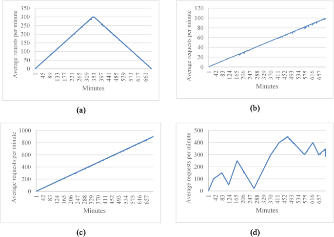
The K6 load-testing tool³⁸ was used to generate HTTP traffic according to predefined workload profiles, enabling evaluation of the system under different request patterns. Workload data were collected by logging incoming requests over a total duration of 697 min; each record represents the average number of requests per second for a one-minute interval.

The resulting dataset was partitioned into three subsets: training, testing, and deployment. While training and testing sets are used to build and validate the prediction models, the deployment set is used during the continuous operation phase to evaluate prediction accuracy in real time and to determine whether the currently selected model remains the most suitable among the available alternatives.

Framework implementation

The framework is implemented using Python 3.0. The framework uses three learning algorithms: Auto-Regressive Integrated Moving Average (ARIMA), Random Forest (RF), and Support Vector Machine (SVM). ARIMA is based on the ARMA model and is specified by three parameters: p, d, and q. p is the number of lag observations representing the series lag period being fitted for prediction, representing the order of the autoregression polynomial. In contrast, d represents the number of times the raw observations are differenced to change the series from non-stationary to stationary. Finally, q signifies the size of the moving average window. Parameters p, d, and q are used by the autoregressive (AR), integrated (I), and moving-average (MA) components of the model. The AR component is an autoregressive model that predicts a variable from its own past values. The integrated part (I) stationaryizes the time series by analyzing differences between observations at different times (I). The moving average (MA) component represents the dependence of an observation on the residual error from a moving average model applied to previous observations.

The SVM model uses support vectors to represent the optimal hyperplane and can solve linear and nonlinear problems. SVM is used in both regression and classification models. It can be applied to time-series forecasting. Still, it needs to transform the dataset into a supervised learning problem using a sliding window of n minutes, where each record contains the previous n minutes of workloads and outputs the predicted workload for the next minute. SVM uses a kernel function to map nonlinear inputs into a high-dimensional feature space. SVM is controlled by a group of parameters, which include the kernel function (K), the cost of misclassification (C), the parameter of a Gaussian Kernel to handle non-linear classification (Gamma), and the margin of tolerance (Epsilon).

Random forest is a supervised machine learning algorithm for regression and classification problems. It can be used for time-series forecasting, but, as with SVM, the dataset must be converted into a tabular form compatible with the supervised learning problem. The algorithm constructs multiple decision trees, each trained on a sample from the dataset. The outputs of these trees are then aggregated via voting or averaging. Random forest is controlled by a group of parameters such as the number of decision trees (n_estimators), the maximum number of features used in splitting a node (max_features), the decision tree maximum depth (max_depth), the minimum number of samples required for leaf node (min_samples_leaf), and the minimum number of samples required to split an internal node (min_samples_split).

The parameters of the learning algorithms are selected dynamically, meaning they are adjusted each time an algorithm is trained. The parameters for SVR and Random Forest models are set using grid search³⁹. For ARIMA, the model parameters are p, d, and q, denoting the AR, I, and MA terms, respectively. The values are estimated using AutoARIMA. The framework analyzes the Partial Autocorrelation Function (PACF) and Autocorrelation Function (ACF) graphs to fine-tune the model parameters. First, the data are examined for trends or seasonality. If the data exhibit a clear trend, the framework performs differencing until the series becomes stationary, starting with first-order differencing (d = 1) and proceeding to higher orders if necessary. Subsequently, the framework analyzes the PACF graph, which displays the partial autocorrelation at different lags. The framework selects p based on the significant lags in the PACF plot. The framework then analyzes the ACP graph to show autocorrelation across different lags. By examining the ACF plot and identifying the last significant lag before it drops close to zero, the framework can adjust the value of q based on the significant lags in the ACF. After determining d, p, and q, the framework can fit the ARIMA model with these parameters. The values are then validated and adjusted during training. Table 4 presents the automatically adjusted parameter values for the different workloads described in Sect. 4.2.

Experimental results with different workload distribution

The experiments apply the four workload patterns discussed in Sect.  3.1 and evaluate the learning models for each workload pattern. First, we analyze the performance of the three models with uniform workloads. Figure 6 shows the prediction values of the three models during the testing phase. As the figure illustrates, during testing, ARIMA shows strong predictive performance, whereas Random Forest initially shows low accuracy; however, the algorithm begins to demonstrate higher accuracy as the load exhibits more uniform behavior. Since a Random Forest is an ensemble of decision trees, each tree is trained independently and initialized with random data and feature subsets. As a result, the initial predictions from individual trees can be inconsistent and may not generalize well. Additionally, SVR shows higher prediction accuracy than Random Forest. The prediction values of the learning models during the deployment phases indicate that all algorithms maintain their prediction accuracy as observed in the test dataset.

Table 5 also shows evaluation metrics for each algorithm based on prediction results during the testing and deployment phases. The table shows RMSE and MAE along with the performance score. It was found that reporting different evaluation metrics can help provide insights into how the models behave under various conditions. As the results show, the ARIMA algorithm has the optimal score value, which indicates that this algorithm is the best solution for the uniform workload. Additionally, all evaluation metrics yield optimal solutions using the ARIMA algorithm. Based on these results, the framework selects ARIMA as the active model and deploys it to production until the framework triggers the retraining phase. Furthermore, the table shows that during the deployment phases, ARIMA still has the optimal score and evaluation metrics, indicating that the framework made the right decision in selecting ARIMA. Since ARIMA performs better in both phases, the framework chooses ARIMA as the active algorithm for the next deployment cycle.

The linear workload represents a steady increase in user requests at a normal rate. Figure 7 shows the predictions of the three models during the test phase. The results indicate that ARIMA exhibits high accuracy, but it fails to predict sudden changes in user requests. In contrast, Random Forest exhibits high prediction accuracy from start to finish, unlike its behavior under the uniform workload (Fig. 6). Similarly, SVR achieves the poorest data fitting compared to the other two algorithms with the linear workload. By the end of the first deployment cycle, the ARIMA score did not exceed the threshold, which led the framework to select it as the active algorithm for the next deployment cycle. Next, if the ARIMA score exceeds the threshold in the next cycle, the framework will pause and retest the threshold before deciding whether to initiate retraining.

Table 6 presents the evaluation results for each model based on the test dataset with a linear workload. As depicted, the ARIMA algorithm achieved the highest score, indicating that it is the best solution for the current workload behavior. Additionally, ARIMA produced the best results for other evaluation metrics. Moreover, it maintained the highest score and evaluation metrics during the subsequent deployment phases. The results demonstrate that ARIMA is the optimal algorithm for the current workload during testing and deployment cycles.

During the deployment phases, all algorithms maintained their prediction accuracy, as seen in the testing phase. However, model performance improves during the second cycle, leading the framework to retain it as the active model. The framework only triggers the training phases when model performance consistently degrades over two successive deployment cycles. As a result, the training process is not repeated frequently, which can consume substantial computational resources. All algorithms improved their prediction performance during the second deployment cycle, with ARIMA remaining the best solution. The algorithm scores shown in the table confirm that continuing to use ARIMA as the active algorithm, without initiating the retraining process, was the right decision.

To evaluate the models with linear workloads at a higher rate, Fig. 8 shows the predictions obtained by the three models on the test dataset. The results indicate that ARIMA achieves high prediction accuracy when the load exhibits uniform behavior. However, it fails to predict sudden changes in user requests. As in its performance with linear workload at a normal rate, the random forest maintains high prediction accuracy throughout the data. Similarly, SVR demonstrates high prediction accuracy as the load increases normally. However, SVR and Random Forest exhibit less curve fitting than ARIMA in this test case.

Table 7 shows that ARIMA has the optimum score and evaluation metrics. Therefore, the framework chooses ARIMA as the active model for the next deployment cycle with a linear workload at a high rate; Random Forest has higher prediction accuracy than SVR. Additionally, all algorithms maintained their predictive accuracy on the test dataset. However, in the second deployment phase, Random Forest achieved the optimal score, with a very small difference from ARIMA, as in the previous experiment at a normal high rate, resulting in negligible differences in prediction accuracy between Random Forest and ARIMA. ARIMA did not exceed the threshold in either deployment cycle. Random workload represents a non-uniform, unexpected change in user request rate. This is the most common type of workload because users’ behavior is non-uniform and varies over time. Figure 9 shows the prediction results on the test dataset. Random Forest shows low prediction accuracy initially, but performance improves; at the peak, when requests begin to change behavior and decrease, accuracy rises. On the other hand, SVR achieves high accuracy from the outset, even with a curve change at the peak. Also, Random Forest shows consistent prediction performance, especially with more data. Also, ARIMA shows high predictive accuracy initially, but after a very short time, it shows poor accuracy.

The results show that SVR achieves the highest performance on random workloads, as reflected by the evaluation metrics reported in Table 8. In contrast, Random Forest exhibits moderate accuracy, while ARIMA performs poorly under highly irregular request patterns. Based on these results, the framework selects SVR as the active model for the subsequent deployment cycle, with its hyperparameters automatically tuned during training. The selected model is then evaluated on the deployment dataset to verify that its predictive quality is maintained under operational conditions.

During the deployment phase, SVR continues to deliver the most stable and accurate predictions across random workload segments. Although Random Forest achieves comparable performance in some intervals, it remains consistently less accurate than SVR, while ARIMA shows persistent degradation. Since the SVR performance does not exceed the predefined retraining threshold, it remains selected for the next deployment cycle, avoiding unnecessary retraining.

Across all workload types, the three models exhibit distinct strengths. ARIMA provides the highest accuracy for uniform and smooth linear workloads, where temporal patterns are stable and predictable. SVR performs competitively in these scenarios but is slightly less accurate. For random workloads, SVR consistently outperforms both ARIMA and Random Forest, while Random Forest offers reasonable but inferior performance.

Each experiment was repeated 20 times to ensure stability of the results. Variance across runs was negligible for the controlled synthetic workloads and is therefore omitted for clarity. For experiments using real-world datasets, standard deviation values will be reported to reflect variability under realistic operating conditions.

Applying the proposed model on a real dataset

After evaluating the framework using simulated workload patterns and verifying its ability to select the most suitable prediction model, the framework was further validated using real-world workload data. To ensure the reliability of the results, each experiment was repeated 20 times for each dataset. The reported performance values represent the average across all runs, while the corresponding standard deviation is included to quantify variability between trials.

The parameter settings used for the FIFA World Cup 2018 workload dataset are summarized in Table 9, including the automatically selected configurations for ARIMA, Random Forest, and SVR models.

The dataset consists of 29 days of hourly workload measurements (696 records, 29 × 24) collected from the FIFA World Cup 2018 website between May 1 and May 29, 2018, representing the number of user requests. The training dataset covers the first 10 days (May 1–10). This training window was selected based on preliminary experiments, which showed that using long training periods reduced prediction accuracy due to the highly dynamic and rapidly changing request patterns throughout the day.

The testing phase was set to 24 h in order to capture the full range of daily workload variations, as request patterns were observed to repeat on a daily basis. Despite this periodicity, the workload remains classified as random because of frequent sudden increases and decreases in request rates.

To evaluate the long-term stability of the model-selection mechanism, the framework was tested over multiple consecutive deployment cycles. As in the previous experiments, model parameters were determined automatically during the training phase. The resulting parameter configurations and performance metrics obtained during the testing and subsequent deployment stages are summarized in Table 10.

Figure 10 presents the prediction results of all three models over the testing phase and four deployment cycles. Random Forest achieves the highest overall prediction accuracy, with only minor fluctuations across cycles that remain below the retraining threshold. SVR also shows strong performance but remains consistently less accurate than Random Forest throughout the deployment phases. In contrast, ARIMA exhibits the lowest prediction accuracy among the three models for this dataset.

The results show that Random Forest achieves the highest performance scores under random workload conditions, indicating that it is the most suitable model for this workload type. SVR also demonstrates good predictive accuracy, but it remains consistently less accurate than Random Forest, while ARIMA performs poorly for highly irregular workloads. Based on these results, the framework selects Random Forest as the active model for the next deployment cycle, with its hyperparameters automatically tuned during training. The selected model is then evaluated on the deployment dataset to verify that its performance is maintained under operational conditions.

Across subsequent deployment cycles, Random Forest continues to achieve the highest scores and evaluation metrics, confirming the stability of the model selection. Since its performance remains above the predefined threshold, retraining is not triggered, allowing the framework to maintain high prediction accuracy while minimizing computational overhead. The gradual improvement in performance over successive cycles is illustrated in Fig. 12.

After validating the framework on real-world data using ARIMA, SVR, and Random Forest, a further experiment was conducted in which ARIMA was replaced by Long Short-Term Memory (LSTM), as ARIMA showed limited effectiveness for random workloads. LSTM is a recurrent neural network designed to capture long-term dependencies in sequential data, making it well suited for time-series forecasting tasks. By incorporating LSTM into the model pool, the framework was further tested under more challenging workload conditions using a neural-network-based predictor.

Evaluating the model with changes in the used algorithms

The proposed framework integrates both traditional and learning-based prediction models. Classical approaches such as ARIMA, SVR, and Random Forest were included because they provide reliable and computationally efficient baselines suitable for real-time deployment. In addition, a Long Short-Term Memory (LSTM) model is evaluated in this section to demonstrate that the framework is not restricted to conventional machine-learning methods, but can also incorporate neural-network-based predictors when deeper temporal modeling is required. The modular design of the proposed MTTD framework allows prediction models—including LSTM and other sequence models—to be added, replaced, or removed according to workload characteristics and available computational resources.

The purpose of this experiment is to evaluate the ability of the framework to operate with different types of prediction models while maintaining low overhead and high accuracy. To balance performance and computational cost, a maximum of three models is used at any time. The experiment was conducted using workload data from the FIFA World Cup 1998 website, which recorded the average number of user requests per second at one-minute intervals. The dataset consists of 1440 min (24 h) of activity, covering the period from May 1, 22:00 to May 2, 21:59.

Training data were taken from May 1, with the size of the training set determined empirically. Since request rates fluctuate rapidly within short time intervals, using excessively long training periods was found to reduce prediction accuracy. The testing phase was set to 100 min, which captures the main variations in request patterns over approximately one and a half hours. The workload is classified as random because of frequent and abrupt changes in request rates during this period. Table 11 summarizes the model parameters used for the FIFA World Cup 1998 dataset.

To further evaluate the adaptability of the framework, the algorithm was tested with additional prediction models to examine its ability to detect performance degradation and trigger retraining when necessary. For this purpose, deployment cycles were allowed to continue until the retraining condition was met. As in previous experiments, model parameters were determined automatically during the training phase. The resulting parameter values and performance metrics obtained during the testing phase and subsequent deployment stages are reported in Table 12.

After the testing phase, the framework selected LSTM as the active model, as it achieved the highest score, as reported in Table 12. In the subsequent deployment cycles, LSTM continued to provide the best overall performance, confirming the validity of the initial selection. This behavior is illustrated in Fig. 11, except for the fourth deployment cycle, where Random Forest achieved a slightly higher score.

During the fifth deployment cycle, the LSTM score exceeded the predefined retraining threshold, which triggered a threshold adjustment to allow one additional evaluation cycle. However, since the score again exceeded the threshold in the following cycle, the framework initiated retraining at the end of the sixth deployment cycle. The retrained models were then evaluated during the testing phase in preparation for the seventh deployment cycle.

Following retraining, SVR achieved the highest performance score and was therefore selected as the new active model. SVR continued to outperform the other models in the subsequent deployment cycles, as summarized in Table 13. Its performance improved consistently across cycles, exceeding the scores obtained before retraining, as illustrated in Figs. 13 and 14.

A comparison between continuing with the previously selected LSTM model and switching to the newly selected SVR model after retraining demonstrates a clear improvement in prediction accuracy. This improvement is shown in Fig. 15, highlighting the benefit of resetting the active model when performance degradation is detected.