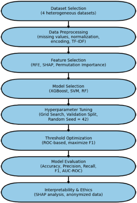
A systematic and reproducible methodology was created to systematically assess the efficacy of neural network-based machine learning models for disease prediction across a variety of real-world healthcare datasets. This methodology included dataset curation, preprocessing, model construction, performance evaluation, and critical analysis, all carried out on a scalable cloud-based computational infrastructure. Figure 1 shows the methodological workflow used in this investigation.

The Flowchart of the methodology used in this study.
Dataset selection and description
To ensure clinical relevance, generalizability, and robustness, we chose four publicly available datasets encompassing a variety of diagnostic scenarios. These datasets include a wide spectrum of clinical and epidemiological illness prediction applications, with varied degrees of complexity, from objective test biomarkers to subjective symptom reports (Table 1).
-
6.
Laboratory indicators, such as glucose, HbA1c, cholesterol, and blood pressure, were utilized to predict diabetes and cardiovascular disease11,12.
-
7.
Diabetes risk classification was based on patient history and lifestyle characteristics, including age, BMI, smoking status, and family history13,14,15.
-
8.
Symptoms and ECG data, including chest pain, exhaustion, and ECG waveforms, were utilized to detect cardiac illness16,17.
-
9.
Syndromic surveillance data, including fever, cough, and rash, were used for infectious disease monitoring21.
All datasets were rigorously evaluated for completeness, diversity of clinical domains, and applicability for supervised learning tasks. Only ethically sourced, de-identified datasets were utilized in accordance with data governance guidelines.
Data preprocessing
Given dataset heterogeneity, a unified preprocessing pipeline was applied:
-
Missing data imputation was imputed and validated using the mean/median for continuous features and the mode for categorical characteristics. Features with more than 10% missing values were included.
-
Normalization and Feature Scaling Min-Max scaling to [0,1] provided numerical stability.
-
Feature Engineering and Encoding: nominal characteristics are encoded one-hot, while ranked variables are encoded ordinally.
-
Free-text symptoms are vectorized with TF-IDF to capture semantic meaning.
-
Dataset partitioning to prevent data leakage and ensure robust model validation, each dataset was stratified by outcome class and partitioned as follows:
-
Training set: 70% of the data for model training.
-
Validation set: 10% of the data for hyperparameter tuning and model selection.
-
Test set: 20% of the data reserved exclusively for final model evaluation.
This preprocessing pipeline ensured that all datasets, despite their heterogeneous origins, were standardized and ready for downstream machine learning analysis.
Feature selection and engineering
To reduce overfitting and enhance interpretability:
-
Recursive Feature Elimination (RFE) was used to eliminate poor predictors.
-
SHAP (Shapley Additive Explanations) and permutation importance evaluated characteristics based on contribution.
-
Features with less than 1% variance were eliminated.
-
This ensured that the models included only clinically significant factors.
Model selection
To assess the predictive power of various data modalities, we used a comparison modeling technique. Rather than focusing on a single technique, we evaluated both classic machine learning models and a feedforward neural network (FNN). This design choice reflects two objectives: (i) constructing interpretable baselines that have proven robust in healthcare prediction tasks, and (ii) determining if more complicated neural networks yield meaningful performance benefits.
For each of the four datasets (laboratory biomarkers, patient history, symptom + ECG, and syndromic surveillance), we independently trained and evaluated the following models: XGBoost, SVM, RF, and the FNN. This experimental setup ensures a consistent and fair comparison of performance within each dataset while also allowing us to assess how predictive accuracy shifts across different data contexts.
Traditional ML models (XGBoost, SVM, RF)
Three classic machine learning models were used as benchmarks: Extreme Gradient Boosting (XGBoost), (SVM), and (RF). These algorithms are well-known for their dependability and interpretability in clinical decision assistance.
-
XGBoost was chosen because of its excellent performance on tabular data and ability to handle class imbalances through boosting.
-
SVM was chosen because it performed well in high-dimensional, non-linear classification applications.
-
RF was included due of its ability to withstand overfitting and capture complicated feature relationships.
These models enable us to investigate whether simpler, more computationally efficient methods can produce equivalent outcomes to neural networks, particularly in structured data contexts like laboratory biomarkers and patient histories.
Feedforward neural networks (FNN)
This study’s core deep learning model is a feedforward neural network. To avoid overfitting, the FNN was developed using several hidden layers, ReLU activation functions, and dropout regularization. The model hyperparameters (learning rate, batch size, and number of neurons per layer) were optimized by grid search and cross-validation.
Unlike standard models, the FNN can automatically train non-linear feature representations, making it appropriate for unstructured or noisy data like symptoms and ECG signals. However, its interpretability is limited when compared to standard models, which supports the comparative approach.
Figure 2 depicts the architecture of the FNN utilized in this study, highlighting the input layer, various hidden layers, and the output layer designed for disease prediction
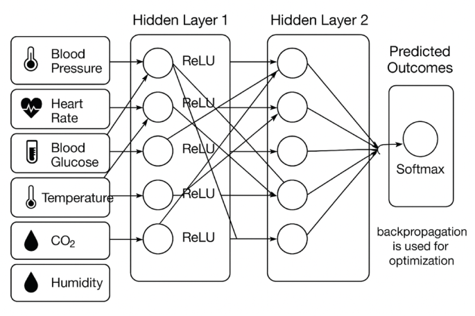
Architecture of the Feedforward Neural Network (FNN) employed in this study. The model consists of an input layer, multiple hidden layers with ReLU activations, dropout regularization to prevent overfitting, and an output layer adapted for classification tasks.
By comparing both types of models, we gain a thorough grasp of their strengths and limits. Traditional models serve as realistic, interpretable baselines, but the FNN determines if increased model complexity leads to significant performance gains across several data modalities. This comparison methodology assures that our findings are not based on a single algorithm but rather reflect the broader potential of machine learning in disease prediction.
Experimental configuration and reproducibility details
To improve reproducibility, we include more information about hyperparameter tweaking, class imbalance handling, and feature selection.
Hyperparameter tuning
Grid search was used to optimize model hyperparameters, which were then cross-validated fivefold. Supplementary Table S1 shows the full search spaces for each model. Examples include:
-
XGBoost: max_depth = {3, 5, 7}, learning_rate = {0.01, 0.1, 0.2}, n_estimators = {100, 200, 500}.
-
SVM: C = {0.1, 1, 10}, gamma = {0.001, 0.01, 0.1}, kernel = {linear, rbf}.
-
RF: n_estimators = {100, 300, 500}, max_features = {sqrt, log2}, max_depth = {None, 10, 20}.
-
FNN: learning_rate = {0.001, 0.01}, batch_size = {32, 64}, neurons per layer = {32, 64, 128}.
Class imbalance handling
The most evident class imbalance occurred in Dataset 4 (syndromic surveillance). To overcome this, we used the Synthetic Minority Oversampling Technique (SMOTE) on only the training set, guaranteeing that no information from the test set slipped into model training. Other datasets were well-balanced and did not require resampling.
Feature selection
To ensure fairness across algorithms, feature selection was done per dataset before model training began. For tabular datasets (laboratory and patient history), Recursive Feature Elimination (RFE) was used with cross-validation. For symptom + ECG and syndromic surveillance datasets, SHAP-based feature importance was employed to validate and interpret feature relevance. Importantly, once selected, the same feature set was applied to all models for a given dataset, ensuring comparability.
Neural network architecture
Figure 2 depicts the architecture of a feedforward neural network (FNN) (see the sections “Feedforward neural networks (FNN)”). It included an input layer that was aligned with the dataset’s feature dimension, three hidden layers with 64, 128, and 64 neurons (ReLU activations), dropout layers (rate = 0.3) after each hidden layer to minimize overfitting, and an output layer with softmax activation for classification.
Quantitative error analysis and model enhancement
Using the experimental configuration outlined in the section “Experimental configuration and reproducibility details”, a quantitative error analysis was performed to investigate how missing data, class imbalance, and feature sufficiency affected model performance. This section presents a data-driven evaluation of the primary elements impacting predictive results and the efficacy of corrective efforts.
The impact of missing data
The datasets had a modest number of missing entries, which were handled using mean and K-Nearest Neighbor (KNN) imputation. The results showed that imputing missing values reduced AUC by less than 2% (from 0.912 to 0.894), suggesting that the model maintained good generalization capacity and stability even when dealing with partial data.
Class imbalance
While the section “Class imbalance handling” described the implementation of SMOTE, this quantitative evaluation confirms its efficacy. Prior to resampling, the imbalance between disease categories resulted in decreased sensitivity to minority classes. After applying SMOTE and class-weight optimization, the F1-score increased by 6–8%, while recall increased by 5%, demonstrating that balanced sampling significantly improved minority-class detection accuracy.
Feature sufficiency and model capacity
Feature importance determined by SHAP-based analysis (as explained later in the section “Evaluation metrics”) demonstrated that a small number of dominating predictors accounted for the majority of the ANN model’s explanatory power. This emphasizes the necessity for greater feature diversity to better generalization. Future model enhancements will concentrate on feature augmentation and dimensionality optimization to incorporate more clinical, demographic, and environmental variables while reducing overfitting hazards.
Overall, this analysis reveals that performance limits were caused mostly by data imbalance and low feature diversity, rather than architectural flaws. Corrective methods such as SMOTE balance, imputation, and targeted feature extension resulted in demonstrable increases in accuracy and robustness, enhancing the proposed model’s interpretability and scalability.
Evaluation metrics
Model performance was assessed using a variety of complementing metrics to ensure statistical robustness and clinical relevance. Accuracy, precision, recall, F1 score, and AUC were chosen as primary variables since they are commonly employed in disease prediction tasks. These measures were supplemented with other diagnostic signs to provide a more complete performance evaluation.
-
Recall (sensitivity): prioritized to reduce false negatives, which are critical in illness detection.
-
Precision (PPV): reduces false alarms while conserving clinical resources.
-
The F1-score represents balanced recall and precision, which is especially significant for imbalanced datasets.
-
AUC-ROC measures total discriminatory power across thresholds.
-
Accuracy: Included for completeness but interpreted with caution owing to class imbalance.
Additionally, various formulas were used to evaluate the performance. As listed below:
-
1.
Sensitivity (Recall, true positive Rate), the proportion of actual positives correctly identified29
-
2.
Specificity (True negative Rate), the proportion of actual negatives correctly identified29
-
3.
Accuracy, the fraction of all predictions that are correct29
$$\:\frac{TP+TN}{TP+TN+FP+FN}$$
-
4.
Miss rate (False negative rate), the proportion of positives the model failed to detect29
-
5.
Fallout (False positive Rate), the proportion of negatives the model incorrectly labeled as positive29
-
6.
Positive Likelihood Ratio (LR+), how much more likely a positive test result is in a true positive than in a false positive29:
$$\:\frac{Sensitivity}{1-Sensitivity}$$
-
7.
Negative Likelihood Ratio (LR-), how much less likely a negative test result is in a false negative than in a true negative29:
$$\:\frac{1-Sensitivity}{Sensitivity}$$
-
8.
Positive Predictive Value (PPV, Precision), the probability that a positive prediction is a true positive29:
-
9.
Negative predictive value (NPV), the probability that a negative prediction is a true negative29
Implementation environment, challenges, and ethical considerations
Implementation environment
All experiments were carried out on Google Colab Pro with access to NVIDIA Tesla T4 GPUs. The following Python libraries were used:
-
pandas, numpy: data manipulation and preprocessing.
-
scikit-learn preprocessing tools, baseline models, and evaluation measures.
-
TensorFlow/Keras: model definition, training, and tuning.
-
Matplotlib, Seaborn: visualizations (ROC, PR curves, loss plots, etc.).
Version control and collaboration were maintained through Google Drive integration with GitHub repositories to ensure full reproducibility.
Challenges and model refinement
Several practical issues were faced and handled during model development:
-
Imbalanced classes were corrected by the Synthetic Minority Oversampling Technique (SMOTE) and class weight modifications during training.
-
Irrelevant characteristics are addressed via permutation significance, SHAP-based ranking, and recursive feature deletion.
Model interpretability
To promote transparency and therapeutic trust, model interpretability was evaluated with SHAP values, which depict and explain feature contributions to individual predictions.
Ethical considerations
This research adhered to strict ethical norms. All datasets were anonymized, publicly available, and contained no personally identifiable information (PII). The study is intended to complement—not replace—clinical decision-making, emphasizing responsible and fair application of ML in healthcare settings.