Figure 3 presents the workflow diagram of the hybrid CFD-ML methodology for optimizing solar thermal collector efficiency. The process begins with CFD baseline model development and experimental validation, followed by parameter range definition for input variables and thermal efficiency output. After generating 935 CFD simulation cases using parallel computing, the workflow splits into two parallel paths: statistical analysis (correlation and parameter impact assessment) and machine learning model development (LR, SVR, and ANN with optimization). Both analytical paths converge to provide comprehensive insights for optimized solar thermal collector performance and thermal efficiency prediction.

Workflow diagram of the present research.
Since MHPA is a proven widely used technique for solar thermal collector for food drying process, a literature paper is selected to establish a baseline CFD model in the study27. The research paper was chosen for two reasons. Firstly, it has been experimentally validated with sufficient measurements, and the secondly, the MHPA design they studied is typically used in many similar solar thermal collectors by recent research25,29.
The CFD model geometry consists of a single heat-collection unit with six key components: glass cover (modeled as “wall” boundary condition), MHPA (length = 1.75 m, width = 0.08 m, thickness = 0.003 m). air duct, and fins, whose detailed dimensions are listed out in Fig. 4(a), which is referenced from literature referrence27.
Solar energy first passes through the glass cover and is absorbed by the MHPA, which conducts the heat horizontally. The aluminum fins conduct this heat, reaching higher temperatures. As ambient air flows through the duct and across these heated fins, the thermal energy transfers from the fins to the air. This heated air can then be used for food drying applications, as shown in Fig. 4(b) and (c).
The study used commercial CFD software ANSYS Fluent Cloud platform with 32 cores for carrying out model simulations. The computational fluid dynamics (CFD) model employs Navier-Stokes equations for incompressible flow. Continuity is enforced through ∇·u = 0, which ensuring mass conservation. Momentum conservation follows:
$$\:\rho\:(\frac{\partial\:\text{u}}{\partial\:t}+\text{u}\bullet\:\nabla\:\text{u})=\nabla\:\text{p}+{\upmu\:}{\nabla\:}^{2}\text{u}+{\uprho\:}\text{g}$$
(1)
where u is velocity, p is pressure, is \(\:{\upmu\:}\) dynamic viscosity, and g represents gravitational acceleration. Energy transport is governed by:
$$\:\rho\:{C}_{p}\left(\frac{\partial\:\text{T}}{\partial\:t}+\text{u}\cdot\:\nabla\:\text{u}\right)=\nabla\:\cdot\:\left(\text{k}\nabla\:\text{T}\right)+\text{S}$$
(2)
where \(\:{C}_{p}\) is specific heat capacity, k is thermal conductivity, and S represents source terms including solar radiation. The buoyancy-driven natural convection employs the Boussinesq approximation for density (ρ) variation:
$$\:\rho\:={\rho\:}_{0}[1-{\upbeta\:}\left(\text{T}-{T}_{0}\right)]$$
(3)
which couples temperature variations to density changes. \(\:{\rho\:}_{0}\) is density, T is temperature, β is thermal expansion coefficient, and T₀ is reference temperature, Turbulence effects are captured using appropriate RANS models with wall functions for near-wall treatment.
The boundary conditions are defined as follows: incident solar radiation is applied as an energy density heat source through the MHPA; the glass cover external surface experiences natural convection with ambient air while its internal surface undergoes coupled radiation-convection interactions, with heat convection governed by the surface heat transfer coefficient; heat conduction occurs at the absorber-MHPA evaporation section interface; the MHPA is modeled as a high-efficiency heat conductor incorporating phase change effects; the air duct system features fluid-solid coupled interfaces between cooling fins and airflow, with air entering at ambient temperature through a velocity inlet boundary and exiting through a free outflow boundary; and the back cover is treated as adiabatic. This configuration comprehensively captures all relevant heat transfer mechanisms: radiation, natural convection, conduction, phase change, and forced convection, referring to the details in Table 1, where the above discussed boundary conditions are summarized accordingly.
It is important to ensure that mesh is refined sufficiently so that model solution does not change further with refinement of mesh. The study is firstly carried out with fewer mesh elements, and then gradually refined mesh until to a point of further mesh refinement does not change the solution.
Polyhedral mesh is generated, and mesh is further refined locally at the areas of interest (e.g., conjugate heat transfer surfaces) to ensure that turbulent flow and heat transfer mechanism is captured.

Schematic view of computational domain of CFD model, with (a) bird view, and example of polyhedral mesh, and zoom-in view of (b) air duct, and (c) fins, MHPA, and glass cover.
Evaluating thermal efficiency
In the present study, CFD model with referring to the experiment set up and numerical model methodology by is developed by using two equation – Reynold Averaged Naver-Stokes (RANS) model, k-epsilon model, to consider the turbulent airflow within the solar thermal collector27. In the reference research27the thermal efficiency has been studied with evaluating a few parameters (e.g., fin spacing, ambient air temperature, and air inlet velocity). However, due to nature that CFD model is expensive to run and requires high performance computing resources, these studies were evaluated with data only under limited design and process conditions. The design and process evaluation of solar thermal collector involves the interaction of many material, design, and process parameters, and thus a more systematic approach that involves large sets of data would help researchers to provide more insights to the thermal efficiency and complex material, design, and process conditions.
Thermal efficiency, η, is an important parameter to evaluate the performance of solar thermal collector, which can be expressed as27:
$$\:{\upeta\:}=\frac{{C}_{p}\dot{m}({T}_{o}-{T}_{i})}{AI}$$
(4)
where \(\:\dot{m}\:\)is the mass flow rate of air, \(\:{T}_{i}\) is the inlet air temperature that enters the solar collector, \(\:{T}_{o}\) is outlet air temperature that enters into the container for drying food, A is the absorber area, I is the solar radiation intensity, and \(\:{C}_{p}\) is the specific heat of air. Thus, in other words, η is the ratio of utilized heat energy that used for heating up the air in the solar thermal collector to the total received solar energy via radiation.
Generating datasets
The effectiveness of machine learning model greatly depends on the selection of appropriate input parameters. Thus, to effectively evaluate thermal efficiency, the material property and process condition need to be carefully chosen to ensure that the developed machine learning model is built upon has relevant and important input parameters for output of thermal efficiency. Thus, six input parameters that describes the material properties and process condition are chosen: Air inlet velocity from ambient environment (\(\:{U}_{i})\), thermal conductivity of metal fins (\(\:{K}_{f})\), heat transfer coefficient of glass cover (\(\:{H}_{g})\), air inlet temperature (\(\:{T}_{i})\), equivalent thermal conductivity of MPHA (\(\:{K}_{m})\), and power density absorbed by the thermal collector (\(\:{P}_{tc})\), which comes from the solar radiation. These input parameters determine numerical condition, which are the specific values of parameters that define the exact mathematical setup for each CFD simulation run. were chosen as input for developing machine learning model. Figure 5 shows the schematic view of the machine learning networks in this study as we discussed above. The chosen input parameters were fed into as input of the system and different machine learning techniques will be applied in the network for calculating the thermal efficiency of solar thermal collector, as shown in Fig. 5.
The above input parameters were identified through a systematic physics-based approach that captures all major heat transfer mechanisms in the solar thermal collector system. The three material properties were selected: thermal conductivity of metal fins (\(\:{K}_{f})\:\)affects heat conduction from the absorber to the air, the equivalent thermal conductivity of MPHA (\(\:{K}_{m})\) determines heat transfer efficiency across the heat pipe system, and the heat transfer coefficient of glass cover (\(\:{H}_{g})\) influences heat losses to the environment. Three operational parameters complete the set: air inlet velocity (\(\:{U}_{i})\) controls the convective heat transfer rate, air inlet temperature (\(\:{T}_{i})\) sets the baseline thermal conditions, and power density \(\:{(P}_{tc}\)) represents the absorbed solar radiation.
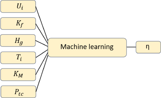
Schematic flowchart of input parameters (e.g., \(\:{U}_{i}\dots\:\:{P}_{tc}\)) to calculate thermal efficiency (\(\:{\upeta\:}\)) by applying machine learning method.
Aside from selecting effective input parameters, an appropriate parameter varying window (defined as the specific range of values within which each input parameter is allowed to vary when generating the CFD simulation datasets) of these input parameters needs to be well defined before generated large set of CFD data because inappropriate parameter varying window will results in unphysical results, and if those results were used in training data sets, the accuracy of developed machine learning model would be compromised or negatively affected.
The selection of machine learning algorithms followed a systematic approach from simple to complex methods to comprehensively evaluate modeling capabilities for the non-linear thermal system. Linear regression (LR) was chosen as the baseline model due to its interpretability and computational efficiency, providing a benchmark for comparing more sophisticated approaches. Support vector regression (SVR)32 was selected for its proven ability to handle non-linear relationships through kernel functions while maintaining robustness against overfitting, particularly valuable given the multi-dimensional parameter space with complex interactions. Artificial Neural Networks (ANN) model33 were implemented as they excel at capturing intricate non-linear patterns in thermal systems through multiple hidden layers, offering the potential for highest accuracy when sufficient training data is available.
Extensive datasets containing 935 numerical cases were modeled by using 32 cores running in parallel by leveraging the available computing resources. The 935 numerical cases were used in the present study through balancing the fact that machine learning models require generating sufficient large number of training datasets and one needs to keep computational cost of running CFD model cases affordable.
Linear regression model
The present study firstly developed linear regression (LR) model as it is the simplest machine learning model. LR model can be categorized into simple LR and multiple LR model34. Simple LR has one independent variable while multiple regression includes several explanatory variables. The basic mathematical form of multiple regression model can be expressed as follows35:
$$y= {b}_{0}+{b}_{1}{x}_{1}+{b}_{2}{x}_{2}+\dots\:+{b}_{k}{x}_{k}+e$$
(5)
where \(\:{b}_{0}\) is a constant term, \(\:{b}_{1}\), \(\:{b}_{2}\),…, \(\:{b}_{k}\) are coefficients of regression terms, and e is sum of errors.
The cost function for LR, Root Mean Square Error (RMSE), which can be written in the below form:
$${\text{RMSD}} = \sqrt{\frac{\sum\:_{i=1}^{N}{\left({y}_{i-}\widehat{{y}_{i}}\right)}^{2}}{N}}$$
(6)
, where N is number of data points, \(\:{y}_{i}\) is observed value.
In addition to RMSE, “R-squared” (R²), referred to as the coefficient of determination, is a statistical metric employed in machine learning to assess the effectiveness of a regression model. It quantifies the degree to which the model accurately represents the data by evaluating the fraction of variance in the dependent variable that is accounted for by the independent variables.
R² can be mathematically expressed by considering the Sum of Squares of Errors (SSE) or the Sum of Squared Residuals (SSR) to the Total Sum of Squares (TSS), which can be detailed as below:
$$\:{R}^{2}=1-\frac{ESS}{TSS}$$
(7)
where, ESS is regression sum of squares:
$$TSS= \sum\:{\left({y}_{i}-\widehat{{y}_{i}}\right)}^{2}$$
(8)
TSS is the regression sum of squares for total:
$$TSS= \sum\:{\left({y}_{i}-y\right)}^{2}$$
(9)
Based on the above description of RMSE and R², one can note that when evaluating the adequacy of a model in relation to a dataset, it is beneficial to compute both the RMSE and the R² value, as each metric provides distinct insights. RMSE indicates the average deviation between the predicted values generated by the regression model and the actual observed values. Conversely, R² measures the extent to which the predictor variables account for the variability in the response variable.
Therefore, the present study will evaluate both RMSE and R² for comparing the performance of different machine learning models. The architecture diagram of LR model is detailed in Fig. 6.

Architecture diagram of LR model in the present research.
Support vector regression model
Support vector regression (SVR) model is chosen in this study as it is popular for addressing regression challenges, primarily due to their ability to model data with non-linear relationships through the use of the kernel trick36. SVR model is frequently utilized with various kernel functions to transform the input space into a higher-dimensional feature space. This transformation introduces non-linearity into the solution, enabling the execution of LR within the feature space37. Taking example of linear functions for best fit function:
$$\:f\left(x\right)=wx+b$$
(10)
With the objective to minimize \(\:\frac{1}{2}{‖w‖}^{2}\) and constraints:
$$\:{y}_{i}-w{x}_{i}-b<\epsilon\:$$
(11)
$$\:{wx}_{i}+b-y<\epsilon\:$$
(12)
where \(\:\epsilon\:\) defines a margin of tolerance, w and b are the weights and bias, respectively .
Figure 7 illustrates the architecture of SVR model used to predict solar thermal collector efficiency. The model transforms the six-dimensional input space, which is through a Radial Basis Function (RBF) kernel with hyperparameters C = 1.0, γ=’scale’, and ε = 0.1. This kernel mapping projects the data into a high-dimensional feature space where a linear regression function can be fitted. The SVR algorithm identifies support vectors (critical data points) that define the regression function within an ε-insensitive tube, allowing for controlled prediction error tolerance and the model ultimately outputs thermal efficiency (η), which is detailed in Figure xx.

Architecture diagram of SVR model in the present research.
Artificial neural networks model
Artificial Neural networks (ANN) model is a class of machine learning algorithms designed to replicate the information processing functions of the human brain. The objective of ANN is the thermal efficiency. Hidden layers are placed in between the objective and input layers for prediction. In the present model, the activation function for hidden layers uses Rectified Linear Unit Function (RELU). The hyperparameters (e.g., L2 penalty parameter) is used as default within scikit-learn library with seven input parameters are input layer and thermal efficiency is the objective38.
ANN model develops rapidly in recent years. ANN can be mathematically considered as a nonlinear regression model \(\:f\left(x\right)=\phi\:(w,\:x)\), where \(\:\phi\:\) is a nonlinear model function and w is the vector that contains the parameters in which x is known as inputs. The basic units of ANN, known as perceptron, can be computed as:\(\:f\left(x\right)=\phi\:({w}^{T},\:x)\), where the nonlinear function \(\:\phi\:\) is called activation function. The training of perceptron model is conducted through the updating of weights as follows39:
$$\:{w}_{i}^{t+1}={w}_{i}^{t}+{\upeta\:}({y}^{m}-\phi\:\left({x}^{T}{w}^{t}\right)){x}_{i}^{m}$$
(13)
where \(\:{\upeta\:}\) is the learning rate.
The generation of comprehensive datasets involved a methodical approach leveraging validated CFD modeling techniques. After establishing a baseline CFD model validated against experimental data from27. Random sampling within these carefully considered parameter ranges was employed to avoid biasing the results, generating 935 distinct simulation cases. Each case represented a unique combination of air inlet velocity, fin thermal conductivity, glass cover heat transfer coefficient, inlet temperature, MPHA equivalent thermal conductivity, and power density for thermal conversion. These simulations, executed in parallel across 32 cores, solved the full 3D thermal-fluid physics with k-epsilon turbulence modeling, capturing the complex interactions between parameters and producing a robust dataset that spans the practical operating space of solar thermal collectors.
As shown in Fig. 8 for the architecture diagram in the present research, multilayer perceptron (MLP) ANN model is used to predict solar thermal collector efficiency. The feed-forward network consists of an input layer with six neurons, two hidden layers with 100 and 50 neurons respectively (both using ReLU activation functions to capture non-linear relationships), and an output layer with a single neuron using linear activation to represent thermal efficiency (η).

Architecture diagram of ANN model in the present research.