Data acquisition and data management
The proposed data was divided into two groups: 44 training samples and 30 testing samples, with an equal split between positive and negative cases. The data of 22 positive glioma patients in the training set and 15 positive glioma patients in the test set were obtained from 2 researches10,11. Additionally, a total of 37 healthy human negative samples from the training and test samples were obtained from IMMUNOSEQ ANALYZER (https://clients.adaptivebiotech.com/).
The raw data from the training samples underwent high-throughput TCR sequencing analysis, resulting in a total of 1,527,623 TCR β sequences. We obtained information about the presence of each sequence in the samples. However, due to the enormous size of the data, it is challenging to incorporate it directly into the classification model. At the same time, cluster identification in high-dimensional sequencing data also faces challenges due to its inherent complexity12. Therefore, we performed feature selection using Fisher’s exact test as we described previously8. We screened 602 TCR β sequences with a P-value less than 0.1, which exhibited a higher correlation with glioma diagnosis, to be used as features for determining glioma.
Classification effects on TCR diversity indices
For these 74 samples, we analyzed TCR diversity, clonality and singleton frequency. According to the common bioindicator system, the article obtains each common immunome sequencing result index corresponding to positive negative samples, such as Clonality index, Shannon diversity index, inverse Simpson diversity index, VJ diversity index, Singleton ratio, and Simpson diversity index these 6 indices.
Of the above indices, the Clonality index is used to measure the extent of TCR clone amplification and to assess the number and proportion of major clones in tumors, with higher values indicating a higher frequency of amplification of some TCR clones. Clonality takes values between 0 and 1, with a value of 0 indicating that each individual is unique and no clone is amplified; a value of 1 indicating that all individuals are copies of the same clone. The index is calculated as follows, where productive unique represents the total number of TCR clones in the sample and diversity is the result of the Shannon diversity index13.
$$ {\text{Clonality}} = 1 – \frac{{{\text{diversity}}}}{{\ln \;({\text{productive}}\;{\text{uniques}})}} $$
The Hvj diversity index is used to measure the diversity of V-J gene combinations of TCR clones in the sample. The index measures the frequency of the ith V-J gene fragment combination use type in the sample by the ratio of pi, thus reflecting the degree of T cell expansion. This index can also be used to reflect the replicative proliferation capacity following stress generated by T-specific recognition of antigen, with higher values indicating a greater degree of clonal amplification, which is calculated as follows14.
$$ H^{\prime} = – { }\sum {\text{p}}_{{\text{i}}} {\text{ln}}\left( {{\text{p}}_{{\text{i}}} } \right) $$
where pi stands for the frequency of the ith V-J gene fragment combination.
The Shannon Index of diversity is used to measure the diversity of TCR clones in the sample. This index incorporates information regarding species richness (the number of different clone types present) and the evenness of the distribution of individuals among these clone types. A higher Shannon index signifies a greater diversity of TCR clones in the sample. The pi in the formula represents the frequency of the ith specific clone type. Thus, the Shannon index considers the number of TCR clone types and the frequency evenness of each clone15.
$$ H^{\prime} = – { }\sum {\text{p}}_{{\text{i}}} {\text{ln}}\left( {{\text{p}}_{{\text{i}}} } \right) $$
where pi here stands for the frequency of the frequency of the ith specific clone type.
The Singleton Frequency is used to represent the proportion of Naïve T cells frequency in a sample and is a metric used to assess the degree of backbone of immune system16. In TCR studies, several studies have shown that the number of singletons is positively correlated with the body’s ability to resist unfamiliar diseases, so this indicator can also reflect the degree of the body’s immune response to the disease. The calculation formula is as follows, where n_1 indicates the number of clone types that appear only once in the sample and n indicates the number of all clone types in the sample.
$$ {\text{Singleton }} = {\text{ n}}\_1/({\text{n}} – 1) $$
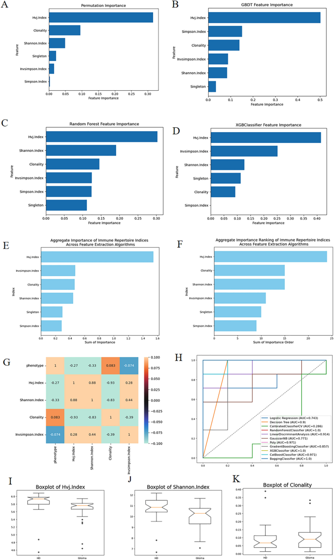
To assess the importance of six indicators, we employed four feature selection methods such as GBDT (Gradient Boosting Decision Tree), RF (Random Forest), XGBoost (Extreme Gradient Boosting), Permutation to rank the importance of this dataset. The corresponding bar graphs are illustrated in Fig. 1A–D. Figure 1E,F represent the sum of importance and sum of importance rank derived from the four feature selection methods respectively. It is evident that the VJ diversity index (Hvj.Index) holds the highest importance, followed by the proportion of monoclonal T cells (Singleton) and Simpson’s diversity index (Invsimpson.Index). Subsequently, Fig. 1I–K display box plots for these three indicators corresponding to positive–negative samples, confirming their distinct differences.

(A–D) show the results of the four feature selection methods. (E,F) are the results of feature selection process of RFECV (Recursive Feature Elimination with Cross-Validation) algorithms, representing the sum of importance and the sum of the ordering of importance respectively. (G) is the correlation coefficient matrix of phenotype and three relevant indicators and one irrelevant indicator. With these three associated diversity indicators, we can attain good classification AUC as is shown in the ROC curves in (H). (I–K) are three box line plots of the three indicators among HD and glioma.
Furthermore, Fig. 1G showcases a correlation coefficient matrix between various indicators and phenotypes. It reveals that the three indicators with higher importance exhibit stronger correlations with phenotypes. Conversely, the indicator with the lowest importance, the Clonality index, demonstrates the weakest correlation with phenotypes.
Figure 1H illustrates the comprehensive ROC (Receiver Operating Characteristic) curves derived from 11 classification algorithms based on the datasets of TCR Diversity Indices and phenotype of the samples. It can be observed that the Random Forest, XGBoost, and Bagging classifiers all achieve a 100% classification AUC value. The three box plots among HD (Health Donor) and Glioma patients in Fig. 1I–K provide further evidence supporting the aforementioned statement.
Binary classification algorithms on TCR sequences
According to our previous two-dimensional classification paper, it has been demonstrated that extracting two-dimensional features from high-throughput sequencing results can improve diagnostic outcomes8. In the context of glioma, the two-dimensional data features extracted from high-throughput sequencing results correspond to a specific threshold of Fisher’s exact test P-value. These features include the total clonetypes and associated clonetypes. The total clonetypes represent the total number of distinct TCRβ sequence species observed in each sample, while the associated clonetypes denote the number of repeated species with associated TCR sequences. With the two-dimensional data above, we built up the classification system with 16 algorithms including neural network algorithms, ensemble learning algorithms and traditional machine learning algorithms. The exact classification result of each algorithm is presented in the Supplementary Table 1.
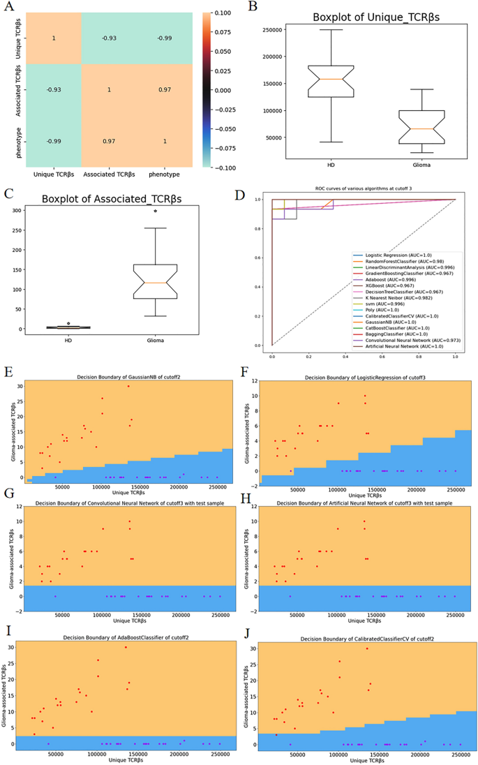
In Fig. 2A, the correlation coefficient plots illustrate the strong correlation between the two-dimensional features and phenotype factors. Specifically, the number of associated clonetypes shows significant relevance to the phenotype, particularly in relation to glioma. This is further confirmed by the box graphs, which reveal a higher number of associated clonetypes in glioma patients compared to healthy individuals. Based on these findings, we construct classifiers using the two-dimensional extracted features from each sample. The data is analyzed using 8 classical classifiers, 4 ensemble learning algorithms, and 2 neural network algorithms. The resulting ROC curves are combined in Fig. 2D, demonstrating that these algorithms achieve excellent classification performance in the two-dimensional data. Some algorithms even achieve an AUC of 1, indicating perfect classification. This highlights the effectiveness of the two-dimensional feature extraction method for diagnosing glioma. In Fig. 2E–J, we present the decision boundaries corresponding to several algorithms that exhibit good classification results.

(A) displays correlation coefficient plots illustrating the relationship between the two-dimensional features and phenotype factors. (B,C) present Box plots showcasing the unique TCRβs and associated TCRβs, respectively, both of which exhibit high relevance to the phenotype. (D) showcases ROC curves for the two-dimensional datasets with a P-value cutoff of 0.001, demonstrating high AUC values. (E–J) shows the decision boundaries of various algorithms at different P-value cutoffs.
Multidimensional classification algorithms on TCR sequences
The multidimensional dataset of TCR β sequences uses 0–1 format data to represent the presence of each sequence in each sample. If the data equals 0, the sequence is absent in the subject, else the sequence exists in the sample. Multidimensional classification algorithms were applied to analyze the tabular data frames of glioma, which contained information on the presence or absence of relevant TCRβs. Several classification algorithms were used, including random forest, support vector machine with linear and polynomial kernel functions, logistic regression, linear discriminant analysis, Bayesian algorithm, GBDT, XGB, and decision tree algorithm.
If the data used to train machine learning models varies in quality, the predicted results may be inaccurate or misleading17. To identify marker sequences specific to glioma while using fewer markers and maintaining high accuracy, feature selection techniques were employed. Fisher’s exact test, a commonly used method in bioinformatics, was utilized for feature selection. By applying different cutoffs for Fisher’s exact test, groups of sequences with varying degrees of relevance to gliomas were identified. These sequences were then incorporated into the classification algorithm system to achieve higher classification accuracy using a reduced number of sequences. This approach allows for the identification of marker sequences specifically associated with glioma. The exact classification result of each algorithm is presented in the Supplementary Table 2.
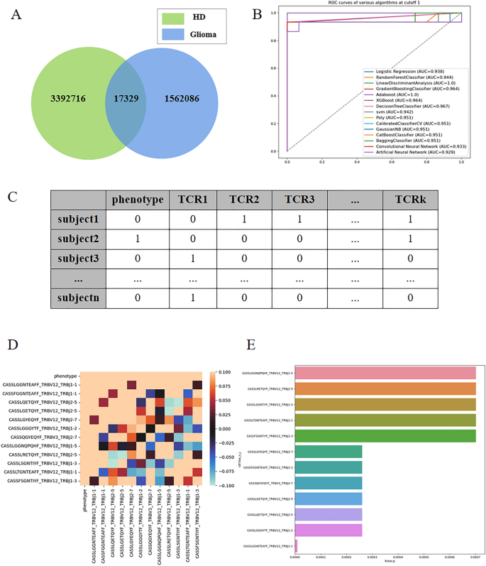
Figure 3A presents a Venn diagram depicting the intersection of sequence species between the healthy and glioma patient groups. It is evident that the sequences in the two groups exhibit high divergence, with only a small fraction being common to both.

(A) presents a Venn diagram illustrating the intersection of sequence species between the healthy and glioma patient groups. (B) shows the AUC (Area Under the Curve) obtained from 602 sequences with a cutoff value of 0.001. (C) displays a tabular dataset with multidimensional columns, where each column represents 0–1 data indicating the presence or absence of TCR β sequences in the samples. A value of 1 signifies the presence of the sequence, while 0 indicates its absence. (D) presents correlation coefficient graphs corresponding to the multidimensional datasets at a P-value cutoff of 0.001. (E) is a bar chart illustrating the importance of the TCR β sequences, with the values corresponding to the P-values of 0.001.
The linear discriminant method achieved the highest accuracy, with an AUC of 100% (Fig. 3B: AUC obtained from 602 sequences with cutoff1 data). In this study, we obtained P-values using Fisher’s exact test and selected TCRβ sequences with P-values less than or equal to 10−2, 10−3, and 10−4, resulting in 39, 12 sequences, and 1 relevant sequence, respectively.
As depicted in Fig. 3C, each column represents binary data (0 or 1) indicating the presence or absence of specific TCRβ sequences in the corresponding samples. We hypothesized that the presence or absence of these sequences is closely associated with glioma status. By analyzing the sequences, we identified a set of TCRβ sequences directly related to glioma and utilized a small number of sequences to accurately predict the disease status.
Next, we applied these sets of sequence data to the 12 classification algorithms mentioned earlier. Notably, when selecting a P-value of 10−3, several classification algorithms also achieved an AUC of 1. Consequently, we narrowed down the factors to these 12 sequence factors. Figure 3D displays the correlation coefficient graphs, indicating that the phenotypes exhibit a relatively high correlation with these sequences, while the correlation with quality control is generally lower.
By utilizing only these 12 TCRβ sequences, we achieved a high prediction accuracy rate. The specific sequences are as follows: CASSLGGNQPQHF_TRBV12_TRBJ1-5, CASSLRETQYF_TRBV12_TRBJ2-5, CASLSGNTIYF_TRBV12_TRBJ1-3, CASLTGNTEAFF_TRBV12_TRBJ1-1, CASSFSGNTIYF_TRBV12_TRBJ1-3, CASSLGYEQYF_TRBV12_TRBJ2-7, CASFGGNTEAFF_TRBV12_TRBJ1-1, CASQGYEQYF_TRBV3_TRBJ2-7, CASLGETQYF_TRBV12_TRBJ2-5, CASSLQETQYF_TRBV12_TRBJ2-5, CASLGGGYTF_TRBV12_TRBJ1-2, CASLGGNTEAFF_TRBV12_TRBJ1-1. Figure 3E presents a bar chart illustrating the importance corresponding to the P-values of these 12 sequences.
Core features’ selection on TCR sequences
Due to computational limitations, we did not perform differential gene analysis on the initial millions of sequences. Instead, we focused on 602 sequences corresponding to Fisher’s exact test threshold of 0.1. Based on this subset of sequences, we explored feature extraction methods that outperformed Fisher’s exact test and identified TCRβ sequences that were more significant for glioma diagnosis. In many cases, the data only describes one chain, and when the α chain lacks data, it is mainly the β chain of TCR. This is a big defect in screening antigen-binding TCR, because the complementary sequence of α-and β-chains determines the specificity of TCR binding18.
Apart from Fisher’s exact test, this study primarily utilized two algorithms for feature extraction: Lasso and RFECV. We employed the Lasso algorithm to select features from the multidimensional data obtained through Fisher’s exact test using threshold values of 0.1, 0.01, and 0.001. In this study, RFECV was combined with nine classification algorithms for feature extraction, and the effectiveness of feature extraction was evaluated using 12 classification algorithms separately. This approach resulted in improved feature extraction, yielding higher classification accuracy with fewer sequences.
Although the two-dimensional features extracted from Fisher’s exact test in Fig. 2 show promising results in distinguishing healthy individuals from glioma patients, we aim to explore additional approaches to identify disease-associated sequences for easier disease diagnosis and future drug development. In the following analysis, we focus on the screening of glioma-associated sequences.
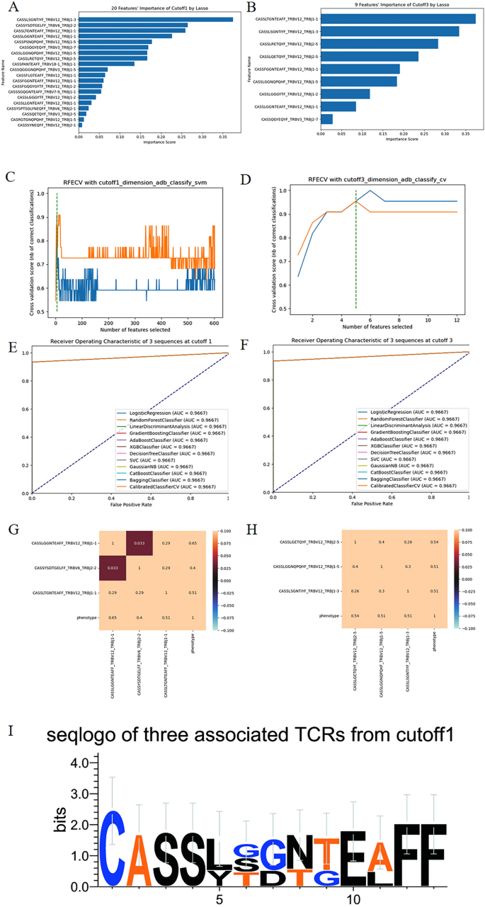
Figure 4A,B illustrate the importance distribution of Lasso with threshold values of 0.1 and 0.001, respectively. We determined that a threshold value of 0.1 yielded an appropriate selection of 19 dimensions for feature selection, while the thresholds of 0.01 and 0.001 resulted in 11 and 9 dimensions, respectively. There are still too many sequences in relative terms.

(A,B) represent the distribution of importance scores obtained from Lasso with threshold values of 0.1 and 0.001, respectively. (C,D) demonstrate the optimal performance of RFECV, indicating that 5 TCRβ sequences yield the highest AUC. (E,F) reveal the ROC curves of the two groups of core sequences and phenotype. (G,H) depicts the correlation coefficient plots of the two groups of core sequences. (I) shows the seqlogo image representing the core 3 TCRβ sequences obtained from the RFECV feature selection algorithm.
While when it comes to the method of RFECV algorithm, as is shown in the Fig. 4C, for the 602 sequences with a threshold of 0.1 for feature extraction, the feature extraction algorithm employed is Adaboost (Adaptive Boosting), and the classification algorithm used is SVM (Support Vector Machine). This approach yields a feature dimension of 5, achieving an AUC of 0.967 and an accuracy of 0.967. The five selected sequences are CASSLGGNTEAFF_TRBV12_TRBJ1-1, CASSYSDTGELFF_TRBV6_TRBJ2-2, CASSLTGNTEAFF_TRBV12_TRBJ1-1, CASSQGYEQYF_TRBV3_TRBJ2-7, CASSLSGNTIYF_TRBV12_TRBJ1-3. Among these five sequences, further extraction using the reject-by-exclusion method identifies CASSLSGNTIYF_TRBV12_TRBJ1-3 and CASSQGYEQYF_TRBV3_TRBJ2-7, while the remaining three sequences, CASSLGGNTEAFF_TRBV12_TRBJ1-1, CASSYSDTGELFF_TRBV6_TRBJ2-2, and CASSLTGNTEAFF_TRBV12_TRBJ1-1, contribute to discriminating the prevalence of glioma. With these three core sequences, high AUC and low correlation degree can be obtained in the Fig. 4E,G.
Using the same method, we analyze the dataset with a threshold of 0.001, which consists of a combination of 12 sequences. As is shown in Fig. 4D, the feature extraction algorithm employed is Adaboost, and the classification algorithm used is CV (CalibratedClassifierCV). This analysis also yields five sequences: CASSLGETQYF_TRBV12_TRBJ2-5, CASSLGGNQPQHF_TRBV12_TRBJ1-5, CASSLSGNTIYF_TRBV12_TRBJ1-3, CASSLQETQYF_TRBV12_TRBJ2-5, CASSLRETQYF_TRBV12_TRBJ2-5. With these five sequences, we achieve an AUC of 0.967 and accuracy, with a sensitivity of 0.933 and specificity of 1. Similarly, by screening one by one, we identify a combination of three sequences that also ensure high AUC values: CASSLGETQYF_TRBV12_TRBJ2-5, CASSLGGNQPQHF_TRBV12_TRBJ1-5, and CASSLSGNTIYF_TRBV12_TRBJ1-3. Meanwhile, Fig. 4F,H demonstrate that the combination of these three less correlated sequences can classify and achieve high classification AUC values. Lastly and not least, Fig. 4I is the seqlogo picture of the core three sequences at cutoff 1 data. Lasso and RFECV are used to extract features, and then several classification algorithms are used to classify the extracted sequence data. The corresponding classification results are shown in Supplementary Tables 3 and 4 respectively.


