
The methodological framework employed in this research is depicted in Fig. 1, beginning with data collection, utilizing key geometric and material properties of concrete slabs as input features. This data was then used to train and evaluate a comprehensive suite of both ML (8 models) and DL (4 models, including a hybrid CNN-LSTM). To ensure a comprehensive and fair evaluation, the selected models were chosen to represent different methodological categories, including linear models (LR, RR, Lasso, EN), ensemble models (RF, GB, XGBoost), and deep learning architectures (CNN, RNN, LSTM, CNN-LSTM). This selection enables a systematic benchmarking framework rather than arbitrary model inclusion and aligns to compare different approaches for predicting (M) and (dr). The performance of each model was rigorously assessed using standard regression metrics, including (R2, MAE, RMSE), to identify the most accurate and reliable predictive model. The overall workflow is summarized in Fig. 1. The workflow explicitly links data preprocessing, model training, and performance evaluation to the main objective of predicting M and dr and comparing different modeling approaches. To improve clarity and avoid ambiguity, a schematic figure was added to illustrate the two main response parameters investigated in this study, M and dr. Figure 2 clarifies the physical meaning of M as a local response parameter associated with slab–column connection behavior, and dr as a global deformation parameter representing the lateral response of the system under seismic loading. In this paper, “punching moment” means the unbalanced moment transferred to the column from the slab at the slab-column joint at the time of punching shear failure. In reinforced concrete flat slab structures under lateral or seismic loading, the unbalanced moment, together with the gravity-induced axial force in the column, causes shear stresses on the critical section around the column. If these stresses exceed the punching shear capacity of the slab, a punching shear failure occurs.

Methodology and model performance evaluation workflow
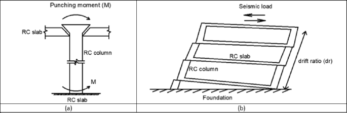
Schematic illustration of the assessed response parameters: (a) punching moment (M) and (b) drift ratio (dr)
Data overview and visualization
The sample used in the paper has 217 records, each having a group of variables that can be used to predict the seismic behaviour of slab-column connections. These records were compiled from published experimental studies, and only specimens with sufficiently complete geometric, material, reinforcement, loading, and response information were included in the final database. A complete list of source studies is provided in the revised manuscript and Supplementary Data. The dataset was divided into 80% for training and 20% for testing, and this split was performed randomly at the individual specimen level over the complete dataset of 217 records, rather than at the study level or test-series level, and all model evaluations were performed on unseen test data to ensure generalization. Figure 3 shows the overall statistics of the main variables to predict the punching shear failure of RC slabs. In Fig. 3, boxplots are interpreted such that the colored boxes represent the interquartile range, the central horizontal line denotes the median, and the whiskers indicate the spread of the data excluding outliers. Negative values reflect the sign convention of the recorded response and represent the opposite response direction rather than invalid physical behavior. These variables are geometric dimensions, material properties, reinforcement properties, and loading conditions. The geometric parameters include L1 and L2 parallel and normal to the loading direction, respectively, slab thickness (h), effective depth (d), and column side lengths (c1, c2). The concrete compressive strength (f’c), tensile strength (ft), and reinforcement yield strength (fy) are some of the material properties that are crucial in determining the mechanical properties of the slab in different load conditions. The flexural ratio (ρ) and compressive ratio (ρ−) of the reinforcement system define the serious influences on the flexural, ductile, and failure behavior of the structural component. Applied gravity load (Vg) indicates the initial vertical loading before lateral loading, and the loading type (LT) indicates the character of the lateral loading, which can be either monotonic or uniaxial cyclic, or even biaxial cyclic. Concerning the output parameters, the dataset will contain the dr, which is the deformation ability of the slab, and the moment at (M), which is the measure of the structural resistance of the ultimate state. Figure 4 introduces a multi-variable analysis of the structural parameters that control the punching shear resistance in RC slabs that incorporates 15 important relationships in a single visual structure. Figure 4a defines the baseline of correlation between (M) and test type because protocol-dependent failure mechanisms are revealed. Figure 4b and c measure the modulating role of slab geometry length parallel and normal to loading (L1) and (L2) in distributing loads. Figure 4d and e indicate the decisive roles played by slab thickness (h) and effective depth (d) in strengthening the sectional rigidity, and Fig. 4f and g reveal that shear forces are focused by the size of columns (c1 parallel to loading, and c2 normal to loading). Moving on to material properties, Fig. 4h and i decipher contributions to the strength of concrete (f′c and ft), and Fig. 4j correlates the reinforcement yield strength (f) to the post-cracking resilience. Figure 4k and l unwind the optimum values of flexural (ρ) and compressive (ρ′) reinforcement ratio in terms of controlling cracks. This analysis leads to a dynamic interaction: the interrelations between Fig. 4m determine moment deformation limits (M) and shear force (Vg) and Fig. 4n superimposes the moment and load transfer (LT) and defines the redistribution of forces when deforming, creating a force redistribution pathway; finally, Fig. 4o plots moment and dr, determining deformation ability. All these panels taken together split up how the interdependence of geometric design, material choice, and load-response relationships determines shear failure, which gives engineers a comprehensive package of tools to draw upon in the prevention of punching shear collapse by designing their buildings optimally in advance. Figure 5 systematically examines the effects of structural parameters on dr in RC slabs; the 15 paramount relationships are combined into one diagnostic structure. The apparent outlier was retained because it corresponds to a valid experimental observation in the compiled dataset and reflects the natural variability of structural response rather than a data error. Its inclusion allows the analysis to better represent realistic response dispersion and to evaluate the robustness of the predictive models under non-uniform data conditions. Figure 5(a) plots dr versus test type and shows that deformation patterns depend on protocol: Fig. 5b and c measure the dependence of deformation distribution on slab geometry length parallel to loading (L1) and normal to loading (L2). Figure 5d and e illustrate the determining factors of slab thickness (h) and effective depth (d) in regulating the stiffness degradation, and the effect of column dimensions (c1 loading parallel and c2 loading normal) on localized defor2mation is revealed in Fig. 5f and g. Moving on to material properties, Fig. 5h and i decode the contribution to the crack propagation resistance by the concrete strengths (f [ and f [ ] ), and Fig. 5j relates the yield strength of reinforcement (f) to the ductility of deformation. Figure 5k and l unveil the capacity of flexural (r) and compressive (r) reinforcement ratio to reduce excessive drifts. The analysis culminates in critical interactions: Fig. 5m correlates (M) with shear force (Vg) to define deformation thresholds; Fig. 5n maps moment against load transfer (LT), exposing deformation redistribution mechanisms; and Fig. 5o ties moment to dr, quantifying collapse progression. Collectively, these panels dissect how geometric configuration, material selection, and force-transfer mechanisms dictate deformation behavior, providing a diagnostic framework for optimizing seismic resilience and serviceability against progressive collapse. Using the analysis of Fig. 6, one can see all the statistical peculiarities of a dataset comprising 217 records and 14 different features, and have the important information to perform a predictive model. The analysis shows that there is a great heterogeneity among variables, with twelve features having great dispersion with standard deviations ranging between 0.17 and 0.24, indicating complex underlying relationships of variables, whereas only two features have low dispersion, with standard deviations of 0.07 and 0.11, indicating deterministic underlying patterns. Extreme value distributions are present by having strong minimum to maximum ranges of 0.00 to 1.00 between all features, and the quartile analysis confirms asymmetric data distributions, with the most significant being in features whose quartile values of between 0.42 and 0.74 are significantly higher than the 0.26 to 0.47 median. The variability profile presented in this case requires strong ML methods since it may have high dispersion values, including a mean of 0.03 and a standard deviation of 0.07, and low variance parameters with a mean of 0.65 and a standard deviation of 0.19, as noted in the variability profile, necessitating regularization methods to reduce noise sensitivity but capture nonlinear relationships. This preprocessing is especially important when dealing with datasets of moderate size, where it becomes possible to efficiently train the models and not lose enough complexity to be able to detect patterns in predictive systems. In Figs. 4 and 5 and a data point located on or near the zero axis does not imply that the corresponding variable does not influence M or dr. Instead, it indicates that, for that specific sample or within that local feature range, the model-estimated contribution is approximately neutral relative to the combined effects of the other input variables.

Comparative analysis of input parameters influencing punching shear failure prediction accuracy. Boxes represent the interquartile range (25th–75th percentiles), the horizontal line within each box indicates the median, and the whiskers denote the data range excluding outliers. Negative values indicate the response direction according to the adopted sign convention and do not imply unphysical behavior


Influence of structural parameters on punching shear resistance: a multi-variable visual analysis: (a) variation of punching moment with test type, (b) slab length parallel to loading (L1), (c) slab length normal to loading (L2), (d) slab thickness (h), (e) effective depth (d), (f) column side parallel to loading (c1), (g) column side normal to loading (c2), (h) compressive strength of concrete (f′c), (i) tensile strength of concrete (ft), (j) yield strength of reinforcement (fy), (k) flexural reinforcement ratio (ρ), (l) compressive reinforcement ratio (ρ′) ,(m) punching moment vs. shear force (Vg), (n) punching moment vs. load transfer (LT), and (o) M vs. dr


Influence of structural parameters on dr: a multi-variable visual analysis: (a) test type, (b) slab length parallel to loading (L1), (c) slab length normal to loading (L2), (d) slab thickness (h), (e) effective depth (d), (f) column side parallel to loading (c1), (g) Column side normal to loading (c2), (h) Compressive strength of concrete (f’c), (i) Tensile strength of concrete (ft), (j) Yield strength of reinforcement (fγ), (k) Flexural reinforcement ratio (ρ), (l) Compressive reinforcement ratio (ρ’), (m) Punching moment vs. shear force (Vg), (n) Punching moment vs. load transfer (LT), and (o) M vs. dr

Feature variability analysis for predictive modeling in structural engineering
ML algorithms
Figure 7 shows a workflow architecture of machine learning to predict punching moment (M and dr). It starts with a stage of exploratory analysis based on heatmaps and statistics to reveal the feature relationships and anomalies. Data cleaning implies KNN imputation, duplicate and type correction. Label-encoded categorical features are used, and through power transformation and min-max scaling, normalized continuous variables. In the feature engineering process, non-informative data (e.g., test symbols) are eliminated, and feature predictors based on the domain are introduced. M and dr prediction are then split on the dataset. Eight linear (LR, RR, Lasso R, EN, SVR) and ensemble (RF, GB, XGBoost) models are trained to predict geometry, material characteristics, and reinforcement information to structural responses. Hyperparameter tuning based on cross-validation guarantees that the model applies to general data, whereas assessment based on experimental data available as holdouts of the dataset determines predictive ability in terms of error measures and residuals. The predictive piping on ML models on punching moments ( M and dr) in a benchmark of an effective workflow in structural vulnerability assessment. The pipeline is a standard that can be replicated and enables performance-based design through the determination of parameterized failure thresholds. Table 2 concludes the efficacy of models as they are valuable in the improvement of the structural performance of slab-column connections under seismic load.

Sequential ML framework for predicting (M and dr ) in RC systems
DL algorithms
DL models are typically applied to large-scale datasets or image-based problems; they are included in this study to investigate their capability in capturing complex nonlinear relationships within structured engineering data. In this context, DL architectures such as CNN, RNN, and LSTM are evaluated to assess whether their representation learning ability can provide additional predictive value compared to traditional ML models. Furthermore, the CNN-LSTM model is explored as a hybrid approach that combines feature extraction capabilities of convolutional layers with the interaction learning potential of LSTM units, aiming to capture complex dependencies among input variables42,43,44,45. The architectures of DL were used to predict severe structural failure processes like (M and dr) in RC systems. In the present study, the DL models were not fed with image-based or time-series data; instead, they were trained using structured tabular input. Each specimen was represented by a one-dimensional feature vector containing the geometric, material, reinforcement, and loading variables. For implementation in the CNN, RNN, and LSTM models, this vector was reshaped into an ordered one-dimensional input sequence, where each feature was treated as one input step/channel in the network. Therefore, the DL models were used to learn inter-feature dependencies within the tabular dataset rather than true spatial or temporal patterns in the conventional sense. This is a computationally intensive model, which follows iterative refinement cycles and uses the adaptive learning properties of neural networks to convert raw structural data into predictive information used in the detection of a collapse. Figure 8 is a more detailed description of our DL model for forecasting these important structural failure mechanisms in the RC systems. This is a computationally heavy procedure in which the adaptive learning abilities of neural networks are utilized via refinement cycles to improve dataset refinement through a carefully executed dataset preparation stage, where extra metadata (test identifiers) has been removed to maximize the relevance of features. Correlation heatmaps are a visual form of interrogative relationship that simplifies querying the relationship between geometric factors (slab dimensions, column sizes), material (concrete strength, relationship between reinforcement and material), and loading features, and simplifies feature selection to be further used in the model. The data is then partitioned into a training and test set, and distributional normalization is done using power transformations and min-max scaling to ensure stability in convergence. Four architectures are then built, each focused on the tasks of spatial stress field in slab column joints, CNN models, time variable loads development CNN, RNN models, crack development pattern, and a hybrid CNN LSTM architecture that combines hierarchies in space with time deformation evolution. Both models have task-specific activation functions (ReLU and tanh) and Adam optimizer, and during training include early stop procedures of 100 or more epochs to stop overfitting and adjust weights backpropagationally as structural responses are predicted and evaluated during training against experimental failure limits. Evaluations on post-training performance are measured by monitoring the R2, MAE, and RMSE performance indicators over the epochs, and the error plots ascertained that the measurements remain stable throughout, as the shear failure response is seen to be recorded. Table 3 compared the performance of these architectures relatively and found that the hybrid CNN LSTM architecture has a better performance in the nonlinear interaction between reinforcement layouts and deformation limits. To further elaborate how both models work, Fig. 7 gives a structural composition of the architectures used in the computational flow of each of the architectures in Figs. 9, 10, 11 and 12. Figure 9 introduces the CNN architecture, and this architecture consists of consecutive convolutional layers that carry with them localized filters to scan the input data and capture geometrical features such as the area of stress concentration or geometric discontinuities in slab column joints. These characteristics are then narrowed down in dimensionality by means of pooling layers, which purvey prevailing information and enhance computational efficiency. This can be further fed directly to one or more fully connected layers, which teach higher-order interactions and produce the final prediction. Figure 10 presents the structure of the RNN, which is specifically developed to deal with sequential data. In this form, the network is in a hidden state, which is updated in an iterative manner by adding new inputs with the memory of past time steps; therefore, the evolving loading patterns or time-dependent material behavior can be modeled. Nevertheless, vanishing gradients frequently tend to make the RNNs susceptible, limiting their capacity to memorize long-term dependencies. To this end, the LSTM network in Fig. 11 builds upon the recurring architecture by including gated memory units, which control the flow of information through an input, forget and output gate which decides which information is retained, discarded or forwards to the next time step, and thus the network to sustain applicable long-term dependencies, including the propagation of cracks or dropped out deformations under cyclical loads. Figure 12 shows the hybrid CNN LSTM model that combines the ability of CNN in extracting spatial features and the ability of LSTM in modeling cases over time. This architecture uses convolutional and pooling layers to first encode non-spatial structural data in meaningful features of space. The processed features are then reworked and input into LSTM layers, learning the temporal development of the said features, e.g., progressive movement or redistribution of stress. This combined model is a well-rounded expression of the structural behavior as it includes such issues as the spatial correlations as well as time-dependent responses, which is an important variable in the accurate depiction of the complicated failure mechanisms of RC in dynamic and nonlinear scenarios.

Sequential DL framework for predicting (M and dr) in RC systems
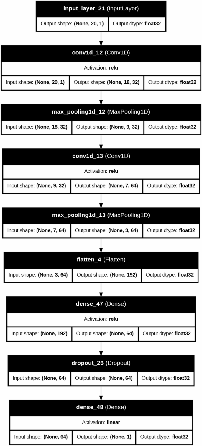
Architecture of the CNN model is used for spatial feature extraction from structural data
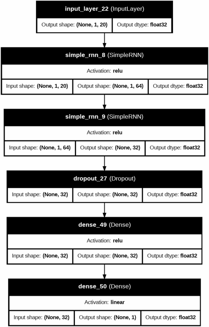
Architecture of the RNN model for modeling sequential structural response

Architecture of the LSTM network for capturing long-term dependencies
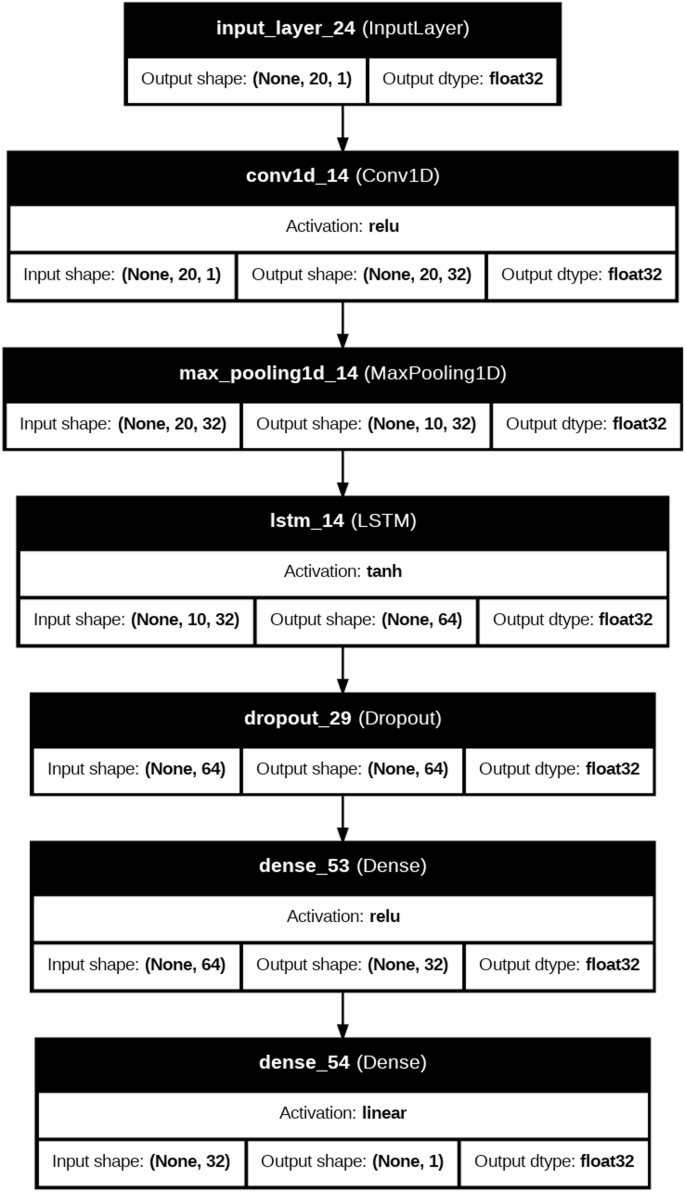
A hybrid CNN-LSTM architecture combining spatial and temporal feature modeling
Experimental setup
The Python programming language was used for the implementation of the proposed ML and DL models. For testing purposes, a Google Collaboratory (Colab) Linux server with Ubuntu 16.04 was used for all experimental testing. This free cloud-based service provides hardware options like Central Processing Unit (CPU), Tesla K80 Graphics Processing Unit (GPU), and Tensor Processing Unit (TPU).
Performance metrics
To strictly assess the predictive power of the models, this paper adopted a set of appropriate statistical measures. All measures were chosen with care, in the sense that they provide complementary insights into model performance: its capability to explain structural behavior, to quantify errors of magnitude, and to describe the statistical nature of predictive discrepancies. The extent of the linear relation between the predicted and actual structural responses was measured by the first metric, R2, which is computed as the ratio obtained by the summation of the products of deviations of the predicted and observed value of means and product of their standard deviations as given in Eq. 146,47. The second measure, MAE, is used to determine the average error rate between actual experimental values and the predictive results. This measure, as explained by Eq. 248,49, is a simple method of quantifying the average size of error that a model generates, without consideration of the fact that the model may be overestimating or underestimating the true outcomes. The third evaluation criterion, RMSE, is used to supplement MAE because it focuses on the effect of greater errors. It is determined by squaring both the error in predictions and the average of the squared values, and then taking the square root of the value, Eq. 3 below50,51. RMSE is especially useful in pointing out the sensitivity of the model to large outliers, which can be present in very nonlinear structural behavior. The mathematical expression of these measures is as follows:
$${\text{R}}^{2}=1-\frac{\sum_{i=1}^{N}({y}_{i}-{\widehat{y}}_{i}{)}^{2}}{\sum_{i=1}^{N}({y}_{i}-\stackrel{\prime }{y}{)}^{2}}$$
(1)
$$\text{MAE}=\frac{1}{n}\sum\limits_{i=1}^{n}\mid {y}_{i}-{\widehat{y}}_{i}\mid$$
(2)
$$\text{RMSE}=\sqrt{\frac{1}{n}\sum\nolimits_{i=1}^{n}({y}_{i}-{\widehat{y}}_{i}{)}^{2}}$$
(3)
where (\(\:{y}_{i}\)) is the actual value, (\(\:{\widehat{y}}_{i}\)) is the predicted value, (\(\:\stackrel{\prime }{y}\)) is the mean of the observed values and (\(\:n\)) is the number of datapoints.
Combining these three complementary evaluation measures, this research develops a strong and effective model for measuring model performance. In conventional ML, the models were trained and evaluated only once, though in the case of the DL models, the models were trained over 100 epochs, and the early stop policies were used to guarantee the best convergence and generalization. This assessment plan provides a significant comparison between the architectures and helps to choose the most reliable models to predict the punching shear failure and drift behavior of RC structures correctly.


