Clustering and machine learning techniques identify air pollution regimes in Greater Cairo

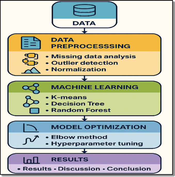
Before describing each methodological component in detail, an overview of the complete workflow is presented in Fig. 1.

Study area and data source

The Greater Cairo Metropolitan Area is one of the most polluted megacities in the Middle East, with a population exceeding 20 million inhabitants. Air quality in this region is strongly influenced by dense traffic, concentrated industrial activity, and recurrent seasonal dust storms transported from surrounding desert regions^21,22.

Data used in this study were obtained from the Copernicus Atmosphere Monitoring Service (CAMS)²³, which provides global reanalysis fields generated through advanced data assimilation systems that combine satellite observations, in situ measurements, and chemical transport modelling²⁴. The CAMS products offer high spatial and temporal consistency, making them particularly suitable for data driven air quality applications.

The dataset covers a continuous two year period from January 2023 to December 2024 and includes both pollutant and meteorological variables: PM₂.₅, PM₁₀, NO₂, SO₂, O₃, CO, near surface air temperature, dew point, wind speed, and surface pressure. CAMS data were extracted at a 3 hourly temporal resolution over the Greater Cairo region and subsequently quality controlled prior to analysis. Following preprocessing, a total of 5,848 complete records were retained, providing a robust basis for subsequent data mining and predictive modelling tasks^25,26. It is important to acknowledge the limitations associated with using CAMS reanalysis data in complex arid urban environments such as Greater Cairo. Previous global validation studies have shown that while CAMS reanalysis products provide consistent large scale atmospheric variability, regional biases may persist when compared against ground based observations, particularly over dust prone and arid regions. These uncertainties are primarily related to aerosol speciation and coarse mode dust representation and may affect absolute concentration estimates (Gueymard and Yang, 2020)²⁷. In this study, CAMS data are not treated as point wise ground observations but rather as a spatially and temporally consistent representation of regional atmospheric variability. Accordingly, the proposed framework focuses on identifying recurring air pollution regimes and relative multi variable patterns rather than relying on absolute concentration thresholds. This regime oriented perspective is inherently more robust to systematic reanalysis biases and remains suitable for supporting short term situational awareness and decision making in data sparse urban environments.

Data preprocessing

To ensure the reliability of the dataset and enhance subsequent model performance, a structured data preprocessing pipeline was implemented²⁴. The procedure consisted of three main stages: (i) missing data assessment, (ii) outlier detection and treatment, and (iii) normalization.

Missing data analysis

The CAMS reanalysis dataset showed no missing values for any of the selected pollutant or meteorological variables²⁴. This completeness reflects the strength of the CAMS assimilation system, which combines satellite and ground based observations to maintain temporal continuity. As a result, the dataset was used directly without applying any imputation procedures, preserving the original information content and avoiding potential artefacts introduced by synthetic values.

Outlier detection and treatment

Outliers were identified using the interquartile range (IQR) method supported by contextual inspection of time series and known pollution episodes as shown in Table 2. The analysis indicated that pollutant variables contained between 4.2% and 8.2% outliers, corresponding mainly to genuine high pollution events, while meteorological parameters exhibited less than 1% extreme values.

For pollutant variables, outliers were retained in order to preserve the representation of real extreme events and avoid underestimating pollution severity²⁵. For meteorological variables, Winsorizing was applied, replacing extreme values with the nearest acceptable bounds. This reduced the influence of potential measurement errors and improved data stability prior to normalization.

Data normalization

All variables were standardized using Z score normalization to ensure a common scale before model training. This method transformed each feature to have zero mean and unit standard deviation according to.

Where X is the original value, µ is the mean of the feature, and σ is its standard deviation.

This transformation prevents variables with larger numerical ranges from dominating the analysis and improves the behavior of algorithms that rely on distance calculations, such as K-means clustering, while also contributing to numerical stability for tree based ensemble models during optimization.

K-means clustering analysis

This subsection outlines the methodology used to apply the K-means algorithm and the procedures followed to identify coherent pollution regimes within the dataset.

Standard K-means implementation

K-means clustering, an unsupervised machine learning algorithm, was applied to identify recurrent air pollution regimes within Cairo’s air quality dataset. The analysis incorporated standardized pollutant concentrations alongside relevant meteorological variables to capture both emission related and dispersion related influences on air quality. Prior to clustering, all features were standardized using Z score normalization to ensure equal contribution to the Euclidean distance metric. The K-means algorithm partitions observations into k clusters by iteratively minimizing the within cluster sum of squared distances, thereby producing compact and well separated groups in the feature space²⁸. This iterative process continues until cluster centroids converge or a predefined stopping criterion is satisfied. MATLAB’s built in kmeans function was employed using multiple random initializations (replicates) to enhance solution stability and reduce sensitivity to centroid initialization. This implementation follows established practices in environmental data mining applications and ensures reproducible and robust clustering outcomes^29,30.

Model optimization using the Elbow method

To determine an appropriate number of clusters for the K-means analysis, the Elbow Method was applied by evaluating the within cluster sum of squares (WCSS) across a range of candidate values of k. This approach assesses the tradeoff between cluster compactness and model complexity by examining how the total within cluster variance decreases as the number of clusters increases³¹.The analysis revealed a clear change in slope at k = 4, indicating that additional clusters beyond this point result in only marginal reductions in WCSS. This inflection point suggests that a four cluster configuration provides an effective balance between capturing meaningful structure in the data and avoiding unnecessary model complexity. Selecting four clusters reduces the risk of arbitrary partitioning and supports the identification of physically interpretable air pollution regimes rather than purely algorithmic groupings. The resulting configuration therefore provides a consistent and interpretable foundation for subsequent regime characterization and supervised classification analyses^32,33. Figure 2 illustrates the Elbow curve, where the observed change in slope at k = 4 supports the selected number of pollution regimes.

Cluster validation and robustness assessment

Although the Elbow method provides a useful heuristic for determining the optimal number of clusters, it does not constitute a formal statistical validation criterion. Therefore, additional complementary cluster validation metrics were computed to assess the robustness of the selected four cluster configuration.

Specifically, three widely used internal validation indices were evaluated for k values ranging from 2 to 8:

• The Silhouette score, which measures the degree of separation and cohesion among clusters³⁴.

• The Calinski–Harabasz (CH) index, which evaluates the ratio of between cluster dispersion to within cluster dispersion³⁵.

• The Gap statistic, which compares observed within cluster dispersion to that expected under a reference null distribution³⁶.

All validation curves are presented in Fig. 3. The Silhouette scores remained above 0.25 across all tested k values, indicating meaningful clustering structure. For k = 4, the Silhouette score was 0.388, reflecting acceptable cluster separation. The Calinski–Harabasz index for k = 4 reached 2099.8, indicating strong inter cluster separation and compactness. Additionally, the Gap statistic remained positive across all candidate k values, confirming that the identified structure deviates significantly from random clustering.

Although different validation metrics may peak at slightly different k values a common phenomenon in unsupervised learning the four cluster configuration demonstrates consistent statistical support while preserving clear environmental interpretability for Greater Cairo’s pollution regimes. Accordingly, k = 4 was retained.

To further assess temporal robustness and regime recurrence, a 50% temporal validation experiment was conducted. K-means clustering was first trained using only 2023 data, and the resulting centroids were subsequently applied to independently assign cluster labels to 2024 observations. Agreement between predicted and independently derived 2024 clusters was quantified using the Adjusted Rand Index (ARI)³⁷, which measures similarity between two partitions while correcting for chance agreement.

The ARI value reached 0.826, indicating strong structural agreement between 2023 and 2024 cluster configurations (ARI ranges from − 1 to 1, where 1 denotes perfect agreement and 0 corresponds to random labeling). This result confirms that the four identified pollution regimes represent stable and recurring atmospheric patterns rather than year specific artefacts.

Decision tree classification

This section presents the supervised classification framework based on Decision Trees, which was employed to evaluate the consistency and separability of the pollution regimes identified by the K-means clustering analysis. In addition to assessing regime separability, the Decision Tree model provides an interpretable rule based structure that links environmental variables to the four identified air pollution regimes.

Base decision tree model

The Decision Tree (DT) algorithm was implemented as a supervised learning approach to evaluate the internal consistency of the regimes derived from the optimized K-means clustering and to develop an interpretable framework for regime membership classification. The model was trained using the standardized dataset, which included PM₂.₅, PM₁₀, NO₂, SO₂, O₃, CO, near surface air temperature, wind speed, and surface pressure as input features³⁸.Cluster assignments obtained from the optimized K-means algorithm were used as categorical target labels, enabling the DT model to learn decision rules that associate specific combinations of atmospheric conditions with each of the four identified pollution regimes.

Hyperparameter optimization process

A systematic hyperparameter optimization procedure was conducted to improve the predictive performance and generalization capability of the Decision Tree model³⁹. Decision Trees provide a high degree of interpretability by mapping threshold based rules between environmental variables and pollution regimes, which is particularly valuable for environmental assessment and decision support applications⁴⁰.

To control model complexity and reduce the risk of overfitting, a range of tree depths was evaluated. Specifically, fourteen maximum depths were tested (10, 15, 20, 25, 30, 40, 50, 60, 70, 80, 90, 100, 120, and 150) to identify an appropriate balance between model expressiveness and stability. In addition to depth optimization, further hyperparameters were examined, including the minimum leaf size (1, 5, 10, and 20) and alternative splitting criteria. These configurations were assessed to determine the most suitable tree structure for capturing the variability of air pollution regimes in Greater Cairo. Model performance was evaluated using a stratified data partitioning scheme, with 70% of the samples used for training and 30% reserved for testing⁴¹, ensuring proportional representation of all pollution regimes in both subsets. Classification accuracy was employed as the primary metric for selecting the optimal Decision Tree configuration, providing a clear basis for comparing model performance across different parameter settings. Although the optimized Decision Tree reached a relatively large maximum depth (90), additional structural diagnostics indicate that the model does not suffer from significant overfitting. The final tree consists of 81 terminal nodes with an average leaf size of 50.54 samples. Furthermore, the training and testing accuracies were 97.36% and 93.10%, respectively, corresponding to a limited train–test accuracy gap of 4.26% points. These indicators confirm that the selected tree depth captures complex relationships in the data while maintaining good generalization performance.

Random forest classification

This section presents the Random Forest classification framework used to evaluate and predict air pollution regime membership, focusing on the ensemble structure, training configuration, and optimization strategy.

Ensemble model framework and configuration

The Random Forest (RF) algorithm was implemented as a robust ensemble learning technique to enhance classification accuracy and model generalization for regime membership discrimination. The model utilized the same standardized input variables as the Decision Tree model, including PM₂.₅, PM₁₀, NO₂, SO₂, O₃, CO, near surface air temperature, wind speed, and surface pressure, with K-means cluster assignments serving as categorical target labels⁴².The ensemble was constructed using bootstrap aggregation and random feature sampling to generate multiple weakly correlated decision trees. Model predictions were obtained through majority voting across the ensemble. An initial configuration of 100 trees was adopted, with Out of Bag (OOB) error estimation enabled to provide an internal and unbiased assessment of model performance.

Advanced hyperparameter optimization and model validation

A comprehensive hyperparameter optimization procedure was applied to determine the optimal RF configuration for classifying pollution regimes in Greater Cairo. Ensemble sizes ranging from 50 to 500 trees were evaluated, alongside variations in the minimum leaf size (1–20) and the number of predictor variables randomly sampled at each split (3–9 features)⁴³. Model performance was assessed using a stratified 70/30 train test split consistent with the Decision Tree evaluation, ensuring balanced representation of all pollution regimes in both subsets. Classification accuracy was employed as the primary selection metric. In addition, permutation based variable importance was computed to quantify the relative contributions of pollutant and meteorological variables to the regime classification process.