Datasets description
The Mammographic Image Analysis Society (MIAS) database is integral to the United Kingdom’s National Breast Screening Program (UK NBSP). This comprehensive collection encompasses 322 mammographic images, capturing both left and right breast views from 161 individuals64. The dataset consists of high-resolution grey-scale images, each with dimensions of 1024 by 1024 pixels, stored in Portable Gray Map (PGM) format. The MIAS database organizes these images into three primary categories based on the nature of the findings: there are 207 normal images, 63 benign images, and 52 malignant images. Moreover, the dataset provides a detailed classification of the images according to the type of background tissue present, which includes fatty, fatty-glandular, and dense-glandular. It also delineates the images by various etiological features. These features encompass calcifications (CALC), well-defined or circumscribed masses (CIRC), spiculated masses (SPIC), masses that are miscellaneous or ill-defined (MISC), architectural distortions (ARCH), and asymmetries (ASYM).
In an illustrative example from the MIAS dataset, Fig. 4 showcases two distinct cases. The first image presents a benign tumor set against a fatty tissue background, characterized by its smooth edges and regular form, indicative of a CIRC etiology. In stark contrast, the second image shows a malignant tumor, also against a fatty background, but marked by an ASYM etiology, distinguished by its blurred boundaries and irregular shape. These comparative visual representations are crucial for elucidating the differences in how benign and malignant tumors manifest in mammographic images.

MIAS breast mammogram images.
The MIAS dataset comprises standard mammographic images and includes a range of abnormal images categorized into benign and malignant types. Within this collection, there are 208 standard images and 114 abnormal images. The abnormal segment is further divided into 63 benign and 51 malignant cases. Each image in the dataset is detailed with a resolution of 1024 × 1024 pixels. For the abnormal images, specific details such as the center point of the abnormality and an estimated radius that delineates the affected area are provided, offering critical insights into the nature and extent of the abnormalities observed.
Data preprocessing
A significant amount of noise is present in the unprocessed images obtained from the MIAS dataset. Data preprocessing is required before model learning to eliminate noise and enhance image quality. Figure 5 illustrates the data preprocessing flowchart. The median filter eliminates noise, and the image is enhanced by contrast-limited adaptive histogram equalization. Following the extraction of the ROIs, a non-breast region is eliminated and rescaled to 120 × 120 pixels. After preprocessing the data, the finalized ROIs with 120 120-pixel borders encompassing 114 abnormal regions were acquired. The relevant ROIs are extracted at a randomized center inside the breast region for normal images, each measuring 120 × 120 pixels. A total of 207 normal and 119 abnormal ROIs (68 benign and 51 malignant). After obtaining ROIs from 207 normal and 119 abnormal images, indiscriminately extracted 72 × 72 pixels patches of each ROI.
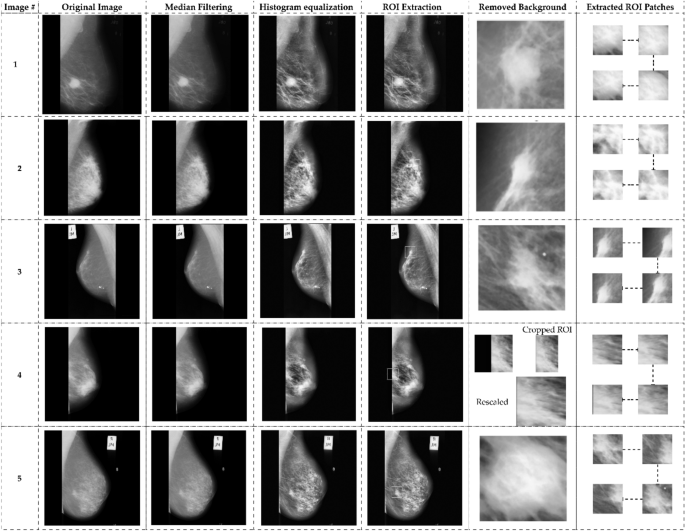
Preprocessing, ROI extraction: (a) original image (b) median filter (2) CLAHE (d) ROIs Extraction (e) ROI cropped (f) Extracted ROI patches to 120 × 120 pixels.
Improved quantum-inspired binary grey wolf optimization
The original Grey Wolf Optimizer (GWO) uses continuous values in the range of 0,1 for the positions of all wolves. In contrast, the Binary-GWO (BGWO) represents the position of each wolf as a binary value, which is calculated using a sigmoid function applied to the GW positions. To solve the unit commitment problem, a quantum-inspired BGWO was introduced18, which proposed an IQI-BGWO to address the selection of feature problems. In IQI-BGWO, the position of each wolf is binary and updated based on a particular qubit vector along with a quantum rotational gate, each wolf having its qubit as well as rotation gate. The \(y\_gate\left( \theta \right)\) Eq. (3) is used for this purpose. While the original GWO updates each wolf position using equations A as well as C, in IQI-BGWO, the location update is dependent on the qubit corresponding to each wolf and the angle θ of each wolf, which is updated based on two probabilistic random γ, ζ values, as demonstrated in the subsequent equations.
$$\left( \theta \right)_{\alpha } \left( {t + 1} \right) = \left( {\upzeta } \right)_{\alpha } \left( {\upgamma } \right)_{\alpha } \sum \left( {\overset{\lower0.5em\hbox{$\smash{\scriptscriptstyle\rightharpoonup}$}}{{\left( {\text{X}} \right)_{\alpha } }} \cdot \left( t \right) – \overset{\lower0.5em\hbox{$\smash{\scriptscriptstyle\rightharpoonup}$}}{\left( X \right)} \cdot \left( t \right)} \right) \cdot 2\pi$$
(10)
$$\left( \theta \right)_{\beta } \left( {t + 1} \right) = \left( {\upzeta } \right)_{\beta } \left( {\upgamma } \right)_{\beta } \sum \left( {\overset{\lower0.5em\hbox{$\smash{\scriptscriptstyle\rightharpoonup}$}}{{\left( {\text{X}} \right)_{\beta } }} .\left( t \right) – \overset{\lower0.5em\hbox{$\smash{\scriptscriptstyle\rightharpoonup}$}}{\left( X \right)} \cdot \left( t \right)} \right) \cdot 2\pi$$
(11)
$$\left( \theta \right)_{\delta } \left( {t + 1} \right) = \left( {\upzeta } \right)_{\delta } \left( {\upgamma } \right)_{\delta } \sum \left( {\overset{\lower0.5em\hbox{$\smash{\scriptscriptstyle\rightharpoonup}$}}{{\left( {\text{X}} \right)_{\delta } }} \cdot \left( t \right) – \overset{\lower0.5em\hbox{$\smash{\scriptscriptstyle\rightharpoonup}$}}{\left( X \right)} \cdot \left( t \right)} \right) \cdot 2\pi$$
(12)
$${\left(\upzeta \right)}_{\alpha }={\left(\uplambda \right)}_{1}.\pi$$
(13)
$${\left(\upzeta \right)}_{\beta }={\left(\uplambda \right)}_{2}.\pi$$
(14)
$${\left(\upzeta \right)}_{\delta }={\left(\uplambda \right)}_{3}.\pi$$
(15)
where θ represents the angle for the quantum rotation gate used in updating the position of each wolf, α, β, and δ denotes the leading wolves in the hierarchy, guiding the search process. ζ and γ are probabilistic random values influencing the rotation angle θ for each wolf, reflecting the stochastic nature of the algorithm.\({\left(\uplambda \right)}_{1},{\left(\uplambda \right)}_{2}\) and \({\left(\uplambda \right)}_{3}\) are random values assigned to each of the leading wolves, affecting the magnitude of ζ for each wolf.
In the context of FFEs, the IQI-BGWO modifies the computation by integrating quantum principles, potentially altering the number of FFEs compared to the baseline GWO. The complexity of FFEs is higher in IQI-BGWO due to the additional quantum computations. Specifically, the fitness evaluation in IQI-BGWO involves quantum state adjustments and rotation, which adds layers to the computational process. Compared to the baseline GWO, where FFEs are direct evaluations of the fitness function, IQI-BGWO requires more computational steps, including the quantum rotation and state update processes.
Random values λ1, λ2, and λ3 are assigned to α, β, as well as δ wolves, and ζα represents the theta magnitude for the α wolf. The corresponding rotation angle is used to rotate each wolf’s qubit vector, denoted as Q, according to Eqs. (16), (17), and (18).
$$\left( Q \right)_{\alpha } \left( {t + 1} \right) = \left( R \right)_{\alpha } \cdot \left( {\left( \theta \right)_{\alpha } \cdot \left( {t + 1} \right)} \right) \cdot \left( Q \right)_{\alpha } \left( t \right)$$
(16)
$$\left( Q \right)_{\beta } \left( {t + 1} \right) = \left( R \right)_{\beta } \cdot \left( {\left( \theta \right)_{\beta } \cdot \left( {t + 1} \right)} \right) \cdot \left( Q \right)_{\beta } \left( t \right)$$
(17)
$$\left( Q \right)_{\delta } \left( {t + 1} \right) = \left( R \right)_{\delta } \cdot \left( {\left( \theta \right)_{\delta } \cdot \left( {t + 1} \right)} \right) \cdot \left( Q \right)_{\delta } \left( t \right)$$
(18)
where Q is a quantum state vector that forms a single qubit. R denotes the rotation operation applied to the qubit vector Q of each wolf, with \({\left(Q\right)}_{\alpha },{\left(Q\right)}_{\beta },\) and \({\left(Q\right)}_{\delta }\) Representing the qubit states of the respective wolves.
$$\left|{\left(Q\right)}_{\alpha }\rangle ={\left(x\right)}_{\alpha }\right|0\rangle +{\left(y\right)}_{\alpha }|1\rangle$$
(19)
$$\left|{\left(Q\right)}_{\beta }\rangle ={\left(x\right)}_{\beta }\right|0\rangle +{\left(y\right)}_{\beta }|1\rangle$$
(20)
$$\left|{\left(Q\right)}_{\delta }\rangle ={\left(x\right)}_{\delta }\right|0\rangle +{\left(y\right)}_{\delta }|1\rangle$$
(21)
where x and y are the coefficients in the superposition of the qubit states, indicating the probability amplitudes for the quantum states ∣0⟩ and ∣1⟩.The initial values of \({\left(x\right)}_{\alpha }\), \({\left(y\right)}_{\alpha }\), \({\left(x\right)}_{\beta }\), \({\left(y\right)}_{\beta }\), \({\left(x\right)}_{\delta }\), and \({\left(y\right)}_{\delta }\) Are set to 1/2. The wolves’ locations are updated based on the probability of the qubit vector being in state |1〉, as follows:
$${\left(X\right)}_{\alpha }\left(t+1\right)={\left(X\right)}_{\alpha }\left(t\right).({y}_{\alpha }^{2})(t+1)$$
(22)
$${\left(X\right)}_{\beta }\left(t+1\right)={\left(X\right)}_{\beta }\left(t\right).({y}_{\beta }^{2})(t+1)$$
(23)
$${\left(X\right)}_{\delta }\left(t+1\right)={\left(X\right)}_{\delta }\left(t\right).({y}_{\delta }^{2})(t+1)$$
(24)
Using a straightforward thresholding operation, the probabilistic values associated with wolves’ positions are converted to binary values that are as follows:
$$\overset{\lower0.5em\hbox{$\smash{\scriptscriptstyle\rightharpoonup}$}}{{\left( {X_{\alpha } } \right)}} .\left( {t + 1} \right) = \left\{ {\begin{array}{*{20}c} {1\; if\; \overset{\lower0.5em\hbox{$\smash{\scriptscriptstyle\rightharpoonup}$}}{{\left( {X_{\alpha } } \right)}} .\left( {t + 1} \right) \ge y_{\alpha }^{2} \left( {t + 1} \right)} \\ {0 \;otherwise} \\ \end{array} } \right.$$
(25)
The first step is to threshold the values of the wolves’ positions to obtain binary values for each feature. As described previously, the threshold is determined based on the qubit probability of state |1〉 for each wolf. The second step is to perform a majority voting scheme for the binary values of each feature among the solutions provided by the α, β, and δ wolves. If most wolves have a binary value of 1 for a particular feature, the final binary value for that feature is set to 1; otherwise, it is set to 0. This procedure results in a binary feature vector \(\overset{\lower0.5em\hbox{$\smash{\scriptscriptstyle\rightharpoonup}$}}{\left( X \right)}\) That represents the selected features for the problem at hand.
1- Use an equation based on the sigmoid function (26) on \(\overset{\lower0.5em\hbox{$\smash{\scriptscriptstyle\rightharpoonup}$}}{\left( X \right)}\) for F \(\overset{\lower0.5em\hbox{$\smash{\scriptscriptstyle\rightharpoonup}$}}{\left( X \right)}\)
2- F \(\overset{\lower0.5em\hbox{$\smash{\scriptscriptstyle\rightharpoonup}$}}{\left( X \right)}\) is compared to a randomized value such that λ.
$${\text{a}}.{ }\overset{\lower0.5em\hbox{$\smash{\scriptscriptstyle\rightharpoonup}$}}{\left( X \right)} = \left\{ {\begin{array}{*{20}c} {1\; F\overset{\lower0.5em\hbox{$\smash{\scriptscriptstyle\rightharpoonup}$}}{\left( X \right)} \ge s } \\ {0\; F\overset{\lower0.5em\hbox{$\smash{\scriptscriptstyle\rightharpoonup}$}}{\left( X \right)} < s} \\ \end{array} } \right.$$
Where s takes on a value from 0 to 1, a sigmoid-function has the following form:
$$sigm\left( p \right) = \frac{1}{{1 + e^{{\left( { – p} \right)}} }}$$
(26)
p indicates the value’s position and takes values ranging from [0 to 1]. The pseudocode of the IQI-BGWO is presented in Table 2:
Improved quantum-inspired binary grey wolf optimization for feature selection
Feature selection serves as a critical step in the realm of machine learning. Its primary role is to trim down the dimensionality of the dataset by selectively retaining features that contribute the most to learning accuracy. This becomes increasingly vital when working with large-scale datasets or tackling machine learning tasks, where computational efficiency and model performance are paramount. This study employs the IQI-BGWO to select features. This algorithm is designed to optimize the subset of features used for training the model, aiming to balance reducing dimensionality and improving classification accuracy. To validate the effectiveness of IQI-BGWO in feature selection, utilize the optimized ISVM classifier as a machine learning model. ISVM is a supervised learning algorithm that uses labeled data to generate a predictive model. It is well-suited for evaluating the quality of the selected features because it is sensitive to irrelevant or redundant features. The primary evaluation criterion focuses on achieving the most minor possible feature set while minimizing the error rate. This dual-objective assessment reduces computational complexity and sustains high model performance. The assessment criteria are encapsulated in a fitness function, framed as a minimization problem, and represented by Eq. 27.
$$fitness=q{P}_{r}\left(M\right)+e\frac{|R|}{|C|}$$
(27)
When reducing the number of features and improving classification accuracy, use the constants e = 1-q and q ϵ 0,1 to use e = 0.01 in this study. R is the length of the subset of features chosen for further analysis, and C is the total number of features in \(q{P}_{r}\left(M\right)\).An in-depth analysis of ten individual experiments conducted using the IQI-BGWO. Each experiment is distinctly numbered for easy tracking, running from 1 to 10. On average, the algorithm achieved a fitness value of approximately 0.0558, though individual trials showed results ranging from as low as 0.0150 to as high as 0.1100. This suggests that while IQI-BGWO is generally effective, its efficiency can fluctuate depending on the specific dataset and initial conditions used in each experiment. In the context of feature elimination, the number of discarded features oscillates slightly between 7 and 9, with an average close to 7.9. This minor fluctuation underscores the algorithm’s ability to adapt its feature selection based on the unique attributes of the dataset. Lastly, the iteration count needed to reach the optimal solution varies noticeably, spanning from a mere 8 iterations to an extensive 58, with the average hovering around 26. This variation hints at the algorithm’s efficiency but suggests that more complex problems might require additional iterations to reach the optimum.
A meticulous account of the performance of the Improved Quantum-Inspired Binary Grey Wolf Optimizer (IQI-BGWO) algorithm over ten separate trials. Each trial is uniquely numbered under the “Trial No.” column for straightforward reference. The general hyperparameters and those specific to the IQI-BGWO algorithm. General hyperparameters include CV, the cross-validation set consistently at 10 for all trials; I, the total number of iterations, fixed at 100; and P.S, the population size, set at 8 across all trials. The objective function to be minimized, denoted by F, is uniformly represented as n ∗ , and its domain, D, is confined to the range 0,1.
Additionally, two weighting parameters for the fitness function, α and β, are set at 0.99 and 0.01, respectively. The “Optimal Iteration” column specifies the iteration count at which each trial yielded its best fitness value, which is then reported under the “Best Fitness Value” column. Special to the IQI-BGWO are parameters like θα, which indicates the θ value for the α wolf in each trial, and Qα, the qubit vector specific to the α wolf. Finally, s represents the threshold the sigmoid function uses for converting probabilistic values to binary. This comprehensive table is a robust tool for evaluating the algorithm’s efficacy and understanding its behavior across different trials.
Improved SVM-RBF
The improved SVM-RBF is a versatile aggregation technique suitable for regression and classification tasks. Unlike conventional statistical-based parametric classification methods, the ISVM-RBF is non-parametric. While SVM is one of the most widely used non-parametric ML algorithms, its performance deteriorates when dealing with large amounts of data. Therefore, the new ISVM-RBF is designed to enhance the efficiency and accuracy of change detection without any assumptions about the data distribution. To handle nonlinear data, the nonlinear ISVM-RBF leverages kernel functions to reduce computational complexity, a technique known as the kernel trick. Popular kernel functions include the polynomial kernel and Gaussian kernel.
In the case of non-linearly separable data, SVM-RBF uses a nonlinear mapping function to convert the input parameters to a higher dimensional space for features., where a hyperplane is constructed to achieve the best classification. This process is recognized as a kernel trick, allowing for efficient computation of the inner product between two vectors without actually computing the transformation. The SVM-RBF can use various kernel functions, but the polynomial and Gaussian kernels are the most commonly used. In this study, the authors focused on the radial basis function (RBF) kernel, a type of Gaussian kernel that has been enhanced for better performance.
The improved ISVM-RBF incorporates two parameters, λ and σ. The parameter σ is used in the execution of the function, and λ is crucial as it determines the compromise between the predicted function along with the minimum fitting error. Therefore, the improved SVM-RBF can be computed as follows:
$$ISVM-RBF=\forall \omega \left(a,{a}_{i}\right)={\text{exp}}\left(-\frac{1}{{\sigma }^{2}}{\left|\left|a,{a}_{i}\right|\right|}^{2}\right)\times \lambda$$
(28)
The first condition for the non-linearity characteristics of SVM-RBF is that it must be symmetric, and the second condition is that it should be capable of ensuring space identification with the problems in the real world, which is the pairwise integrating potential. Equations 28 and 29 establish these two conditions, where ∀ω*(\(a,{a}_{i}\)) represents the improved SVM-RBF attributes, as well as the variant function, is represented by ∀ω .
$$\forall \omega \left(\left(a,p\right)=\left(\varphi \left(a\right).\varphi \left(p\right)\right)\right)$$
(29)
$$\forall \omega \left(a,p\right)-\left\{\varphi \left(a\right).\varphi \left(p\right)\right\}=\left\{\left(a\right).\varphi \left(p\right)-\forall \omega \left(a,p\right)\right\}$$
(30)
The one verses all technique can integrate binary classifiers with SVM-RBF. In the context of a K-classification issue, the one verses all approach generates a single binary classifier for each class. In this method, all samples of a particular class have y = 1, and all samples of the remaining (k-1) classes have y = 0. Therefore, there will be k-binary classifiers in total. All k binary classifiers will be executed to classify new data x, and it will be classified into the class of i, providing the most significant probability as well as classification result.
The choice of the SVM-RBF as the classifier in this research is grounded in its exceptional ability to manage nonlinear data through the kernel trick. This approach is crucial for datasets where the relationship between features is complex and not linearly separable. The kernel trick allows the SVM-RBF to project data into a higher-dimensional space, facilitating a more nuanced and effective classification boundary than linear models could achieve. This capability is particularly advantageous for complex classification tasks where the intricacies of data relationships need to be accurately captured.
The SVM-RBF framework is also valued for its robustness in handling high-dimensional data spaces. It maintains performance even when the dataset features are large compared to the number of samples, a scenario where many models tend to overfit. Overfitting compromises the model’s ability to generalize to new data, but the SVM-RBF’s structural design inherently avoids this pitfall, thus ensuring more reliable predictions.
Moreover, the improved version of SVM-RBF, or ISVM-RBF, introduces enhancements that address some of the conventional SVM limitations, such as scalability and computational efficiency. These improvements are particularly relevant when dealing with large datasets. By fine-tuning the model parameters, λ and σ, the ISVM-RBF achieves a balance that enhances the model’s performance and computational efficiency. This balance is crucial for practical applications where accuracy and processing speed are essential.
While other classifiers like XGBoost, AdaBoost, and Random Forest are effective in various scenarios, their appropriateness depends heavily on the specific characteristics of the problem and the data at hand. For instance, while Random Forest is adept at handling datasets with many features and can deal with nonlinear relationships, it may not provide the same level of performance as SVM-RBF in situations where the separation margin between classes in the feature space is minimal. Therefore, the selection of ISVM-RBF for this study was strategic, aimed at leveraging its specific strengths in handling the unique challenges posed by the dataset. This included its proficiency in dealing with nonlinear separability and high-dimensional spaces and its ability to avoid overfitting, thus ensuring that the model remains effective and reliable when applied to new and unseen data.
ISVM-RBF optimization
The optimal values of parameters are crucial for achieving a superior classification rate while training the SVM classifier. Optimization algorithms such as IQI-BGWO and BGWO are employed with the SVM classifier to obtain these ideal values. This results in the optimal classification accuracy for the classifier. The proposed system is described in Fig. 6. Once the optimal parameters of the SVM are obtained, the dataset is trained to obtain the learning model, which is subsequently utilized to anticipate the test data and obtain the highest possible classification accuracy. Instructions for implementing the recommended optimal SVM model are as follows:
-
1.
First, generate a random population of GW’s. Optimal ISVM performance depends on balancing two parameters; therefore, data on every individual is stored in a two-dimensional array. The next step is to determine the fundamental IQI-BGWO parameters. Train the ISVM and assess the fitness of each search agent.
-
2.
The IQI-BGWO-SVM’s fitness function is created following its classification accuracy throughout cross-validation. This study takes advantage of the K-fold CV method, which can assess ISVM’s generalizability accurately. This work uses cross-validation at three different levels: 5, 10, and 15 CV, along with the fitness function developed based on the performance of the training set in the CV.

Flow chart of IQI-BGWO-SVM.
When reducing the number of features and improving classification accuracy, use the constants e = 1-q and q ϵ 0,1 to use e = 0.01 in this study. R is the length of the subset of features chosen for further analysis, and C is the total number of features in \(q{P}_{r}\left(M\right)\).
-
3.
In step 3, when an initial population has been generated using data set samples as input to the model, the fitness of every one of them is determined using the fitness function. Their fitness levels are ranked from highest to lowest to determine which three grey wolves have the greatest hunting skills. These wolves are then given the names α, β, and δ.
-
4.
The location updates of all the grey wolves will be coordinated when the initial values of α, β, and δ have been chosen. This results in the formation of a new population of grey wolves in which the roles of the individuals have shifted. After that, an assessment and computation of every individual’s fitness level is carried out. The population is broken up into α, β, δ, and ω accordingly. The preceding process will repeat indefinitely if the maximum possible number of iterations has not been attained.
-
5.
After iteration, the model will output the optimal solution, substituting it into ISVM to create an optimal classifier. The effectiveness of the hybrid classification framework is evaluated next using test set samples drawn from the whole dataset.
Performance metrics
To assess the classification performance of the IQI-BGWO–SVM and BGWO–SVM models, this study employs a set of established performance metrics, which are pivotal in machine learning and statistical analysis for evaluating the efficacy of classification models65,66,67. The chosen metrics are Accuracy, Specificity, Sensitivity, Error Rate, and Matthew’s Correlation Coefficient (MCC), each serving a distinct purpose in quantifying model performance.
Accuracy (ACC) represents the proportion of correctly classified samples (both true positives and true negatives) to the overall sample count. It is calculated as:
$$ACC=\frac{{\text{TP}}+{\text{TN}}}{{\text{TP}}+{\text{TN}}+{\text{FP}}+{\text{FN}}}\times 100\mathrm{\%}$$
(31)
where (TP) is true positives, (TN) is true negatives, (FP) is false positives, and (FN) is false negatives.
Specificity (SPC) measures the proportion of actual negatives correctly identified as such (true negatives) and is vital for assessing the model’s ability to identify negative cases. It is computed as:
$$SPC=\frac{{\text{TN}}}{{\text{TN}}+{\text{FP}}}\times 100\mathrm{\%}$$
(32)
Sensitivity (SEN)indicates the model’s ability to identify positive cases correctly. It is the proportion of actual positive samples that are correctly classified as positive:
$$SEN=\frac{{\text{TP}}}{{\text{TP}}+{\text{FN}}}\times 100\mathrm{\%}$$
(33)
Error Rate (E.R) calculates the proportion of all incorrect predictions (both false positives and false negatives) to total predictions, giving an overall measure of the misclassification:
$${\text{E}}.{\text{R}}=1-0.5\times \frac{\mathrm{SEN value}+\mathrm{SPC values}}{100}\times 100\mathrm{\%}$$
(34)
Matthew’s Correlation Coefficient (MCC) provides a balanced measure that considers true and false positives and negatives, suitable for imbalanced datasets. It is defined as:
$$MCC=\frac{{\text{TP}}\times {\text{TN}}-{\text{FP}}\times {\text{FN}}}{\sqrt{(TP+FP)(TP+FN)(TN+FP)(TN+FN)}}\times 100\mathrm{\%}$$
(35)
These metrics are selected based on their ability to view the model’s performance comprehensively. Accuracy offers an overall effectiveness rate, while Specificity and Sensitivity give insights into the model’s ability to identify each class correctly. The Error Rate provides a direct measure of the model’s misclassification. MCC offers a balanced metric considering all aspects of the confusion matrix, making it particularly useful for evaluating models on imbalanced datasets.
In addition to Accuracy, this study includes Specificity, Sensitivity, Error Rate, and MCC to ensure a holistic evaluation of the classification models, accounting for various aspects of performance that single metrics like Accuracy cannot fully capture. These metrics collectively enable a detailed assessment of the models’ ability to effectively classify and distinguish between different classes, considering both the positive and negative instances.