David Gerbing of Portland State University’s School of Business introduces lessR, a tool designed to facilitate professional-quality data visualization and data analysis without any programming requirements.
I developed lessR to simplify the process of getting professional quality data visualization and general data analysis for free and with minimal effort. Download R and its easy-to-use analysis environment, RStudio, for free. Quickly learn how to set up and use the environment, and see many examples, through the same website I developed for my students. No programming required, just a simple function call.
In the first article of this series, we introduced a wide range of data visualizations. Second highlighted time series forecast. This article explores machine learning to build predictive models not from historical data of the same variable (time series), but from existing data values of other variables, called predictor variables. The variable predicted by the model is called the target variable.
Here we discuss the classic early forms of supervised machine learning: linear regression for predicting the value of a continuous variable and logistic regression for predicting the value of a categorical variable with two categories (or groups). Although there are many forms of supervised machine learning, most of which have been developed relatively recently and perform better than traditional versions in certain situations, these versions are still widely applicable and are a good introduction to the topic.

data
We usually read data named d into R. This data serves as the default data name for analytic functions. and less R In the Read() function, enter the location of the file on your computer or on the web, enclosed in quotation marks, as follows:
d <- Read(“https://dgerbing.github.io/data/Employee.xlsx”)
The file name can refer to an Excel sheet, a text file, or many other data formats, as in this example. To refer to a file, leave the quotes empty. read(“”).
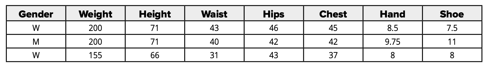
Below are the first 3 lines of 340 actual body measurements from a company that sells clothing online.
Regression analysis
Suppose you don’t know a person’s weight, but you have other measurements such as height and waist size. A regression analysis predicts weight (pounds) from two predictor variables: height (inches) and waist size (inches). Given the data above, the first step is to estimate a regression model to predict the weights using the following formula: less R Function reg().
reg(weight ~ height + waist)
This single instruction produces a thorough and comprehensive regression analysis with several visualizations displaying various regression statistics and diagnostic criteria. Here we only consider the basic model with three numerical coefficients estimated from the data.
Predicted weight = -327.07+5.325(waist) + 4.522(height)
Enter a person’s waist size and height into that equation and calculate their predicted weight.
One of the visualizations is a scatterplot matrix, which shows the correlation and scatterplot between every pair of variables. The goal is for each predictor to be relevant, highly correlated with the weights, which is our target here, relatively unique, and not highly correlated with other predictor variables.
Logistic regression
Logistic regression is required because weight is a continuous variable, but gender in these data is categorical with only two values, M and W. Here, we predict gender based on hand size. First estimate the model
Logit (gender ~ hand)
The output includes a 2-by-2 classification table of correct and incorrect classifications, with a correct prediction accuracy of 88.2%. Here, gender 0 is M and gender 1 is W.
The prediction rules are simple. Predict M if the hand size is greater than 8.408 inches, W otherwise.


The following visualization uses two Y axes to show details. The left Y-axis shows the probability that a person’s gender is M, and the right Y-axis shows the probability that the person’s gender is M or W. The vertical dashed line is the hand size threshold for predicting M or W, 8.408. The threshold 8.408 is the point at which the probability of either M or W is 0.5. Hand sizes much larger than about 9.5 result in probabilities close to 1 in M. Similarly, a hand size less than about 7.2 means that the probability of M is close to 0, which means that the probability that the person is W is close to 1.
There are many aspects to discuss about regression analysis and logistic regression, and even more to discuss regarding the output from the corresponding lessR functions, but this short presentation will provide you with the basic knowledge, reading statements, and two simple function calls to do two types of serious, easy, and free model building.


