

Research Design and Data Collection
This study adopted a cross-sectional description design using a convenient sampling method. Microscopic images were collected using a CX41 biological microscope (Olympus, Tokyo, Japan) from 1,582 vaginal secretion samples. These catered to 1,582 women over the age of 18 who were diagnosed with vaginosis at University Medical Center Ho Chi Minh City between January and August 2024. The mean age of these women was 33.7 ± 10.2 years. This study did not collect any individual identification information and provided written informed consent for image collection from all participating women. This study was conducted in accordance with relevant guidelines and regulations for studies involving human subjects and was approved by the Biomedical Research Ethics Committee at the University Medical Centre in Ho Chi Minh City, Vietnam (137/2024). Gynecological examinations, collection of vaginal secretion samples using sterile swabs, and subsequent relocation to the lab were carried out independently of the research team by specialized obstetricians and gynecologists. In some cases, additional diagnostic techniques such as gram staining, pup smears, or fine needle aspiration (FNA) were used as routine procedures. Treatment decisions were based on vaginal discharge test results, symptoms, and gynecological examinations. In the laboratory, vaginal discharge samples were prepared as wet mount specimens, examined under a CX41 biological microscope, and microscopic images were captured for analysis by experienced technicians. After consultation with laboratory engineers, the research team collected microscope images and assigned image classifications. Among the 1,582 vaginal secretion samples analyzed in this study, classification based on the presence of pathogens revealed different proportions between different groups. Specifically, 35.4% of the samples were related. Gardnerella vaginalis (Group C), identified through cues in wet mount preparation. 31.6% are related to fungal infections and are primarily responsible Candida Species (Group F); 33.0% contained a diverse pathogen Trichomonas vaginalishuman papillomavirus (HPV), and various bacterial species (Group B). In particular, bacterial pathogens, as the primary agent in Group C or as part of the mixed pathogens in Group B, were present in 68.4% of the samples, indicating that bacteria or other bacteria constituted the majority of cases studied. This high prevalence of the presence of bacteria, especially in Group C, highlights the importance of accurate diagnostic methods for conditions such as bacterial vaginosis (BV). Group C serves as a key indicator of BV identified through the cuing cells of a standard screening technique, wet mount microscope, but the diagnosis of BV cannot rely solely on this finding. Conclusive confirmation requires additional clinical or clinical disease assessments, such as Amsel's criteria and Nugent's scoring system, to ensure diagnostic accuracy. This study focused specifically on screening groups B, C, and F, but did not incorporate routine exclusions for other sexually transmitted diseases (STIs). Chlamydia or go disease. However, in a clinical setting, these pathogens still require targeted diagnostic testing if symptoms or risk factors suggest a potential presence. A total of 3,164 RAW images were collected from these samples and used a 40x objective magnification CX41 biological microscope. All images were systematically captured via a microscope's integrated camera to ensure standardized quality and consistency across the dataset. During preprocessing, these were resized to 800 x 800 pixels. This is the step taken to normalize the input dimensions of model training and improve computational efficiency. Therefore, they were divided into three groups based on the cause of vaginitis: group C (Gardnerella vaginalis), group F (fungal vaginitis), and group B (other pathogens). Figure 1 outlines the methodological workflow of data processing and analysis in the research. This procedure began with a vaginal secretory image dataset that was preprocessed using a photodirector to standardize image quality. Following preprocessing, the dataset was split into training, validation, and test subsets. A pre-trained MobileNETV2 architecture was adopted and model training was carried out on the training set. We then used validation and test sets to assess the performance of the model. A predefined optimization metric and iterative training loop led by end conditions was implemented to improve the model. This process ensured systematic optimization and culminated in the generation of final classification results.

A summary of survey data and methods.
Pre-processing of images
All microscopic images were subjected to standardized preprocessing using a photodirector before the dataset was trained, validated, and divided into test subsets. This preprocessing was applied uniformly across the dataset to ensure consistent input data for deep learning models and to improve image quality for improved feature extraction. Included pre-processing steps:
Image sharpening
To enhance the clarity of the microscopic details, sharpening was applied to address the lack of inherent details of raw microscopic images. This step was important to improve the visibility of key diagnostic functions such as fungal structure, cues and inflammatory cells.
Image size change
All images were resized to uniform dimensions of 800 x 800 pixels (Figure 2). This standardization was essential to optimize computational efficiency and ensure consistent input dimensions for MobileNETV2 models without losing important diagnostic information.
Rotation and adjustment
Images were rotated 90°, 180°, or 270° to create variations of the same sample. This allowed the model to learn to recognize features from different angles.
Light and color adjustment
Adjusting illumination and contrast was done to standardize illumination and contrast inconsistencies caused by various microscope conditions, improving the model's ability to learn from more uniform data.
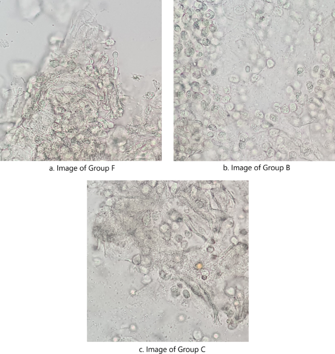
Representative 800 x 800 pixel images of vaginal secretion samples from groups B, C, and F.
Data division
Following the preprocessing stage, which was applied uniformly across the dataset, the images were split into three subsets: 80% in training, 10% for validation, and 10% for testing. For model training, a pre-trained MobileNETV2 model was first used, trained on an Imagenet dataset (including over 1.2 million images from 1,000 categories). MobileNETV2 was chosen for efficient management of computational and memory resources, particularly in mobile environments.
Mobilen ETV2 Architecture and Training Process
The Co-Inovation of MobileNETV2 is located in the main building block (Figure 3), extending the input channel via 1×1 convolution, applied lightweight 3×3 depth convolution, extending the back-projected features using linear (non-RELU) 1×1 layers.19. Unlike traditional residuals, the shortcuts connect narrow bottleneck layers and bypass the extended intermediate representation to store memory. MobileNETV2 uses a method that reduces processing time by focusing on key image features, making it eight times faster than traditional approaches. Linear bottlenecks prevented loss of relationship-induced information in low-dimensional spaces and maintained a critical function. When combined with optimized training, this design achieved high accuracy under strict computational constraints, allowing for efficient mobile deployment.

Mobilenetv2 main building blocks.
The model was initially trained at a learning rate of 0.001, with batch size starting at 10 and increasing to a maximum of 128 per loop. Training continued with up to 100 epochs and was stopped early based on the accuracy metrics of the validation set to prevent overfitting. Two different accuracy metrics were used to comprehensively assess the performance of the model: trace academia and macro acceleracy20. The trace accuracy was calculated globally by taking into account the total number of instances correctly classified across all classes, dividing them by the total number of instances. This metric provided an overall measure of the effectiveness of the model in classifying instances regardless of class distribution. Conversely, macro accuracy was calculated by first determining the accuracy of each class individually and then averaging the accuracy of these classes. The macro accuracy provided an unweighted average of the accuracy per class, giving equal importance to each class regardless of the frequency of the dataset. These metrics were calculated after each loop for both validation and test sets. Training stopped when both the validation and test sets were above 0.80 for both the trace and macro precision. Accuracy and recall were then calculated for each group (b, c, f).
Training and evaluation
During training, the batch size gradually increased from 10 to 128. If the validation set achieved a trace accumulation ≥0.80 and a macroaccaccalci ≥0.80, training continued until similar metrics were met or screened on the test set. The final model achieved the following accuracy scores: Validation Set – Microbial Abundance: 0.83, Macro Acacity: 0.87; Test Set – Micro Acacacity: 0.85, Macro Acacity: 0.88; Training Set – Micro Acacity: 0.89, Macro Acacity: 0.91.
Model performance evaluation
Given the unbalanced nature of the vaginitis classification dataset, accuracy alone was not sufficient for model evaluation. Therefore, in this study we also adopted Precision-Recall curves and F1 scores.
Precision Recovery Curve: This curve measured the model's ability to correctly identify the cause of vaginitis while minimizing false positives. Accuracy indicates the percentage of true positives among predicted positives, and the recall reflects the percentage of actual positives correctly identified.
F1 Score: As the accuracy and recall average of harmonic mean, F1 Score provided a balanced assessment of model accuracy, especially in the binary classification task. An F1 score above 0.75 indicated the effectiveness of the model in identifying true positives, while minimizing diagnostic errors.
$$\:\text{f}1=2\times\:\frac{\text{p}\text{r}\text{e}\text{c}\text{i}\text{s}\text{i}\text{o}\text{n}\:\times\:\:\text{r}\text{e}\text{c}\text{a}\text{l}\text{l}}{\text{p}\text{r}\text{e}\text{c}\text{e}\text{c}\text{i}\text{s}\text t{i} \text {o}\text {n}+\text {r}\text {e}\text {c}\text {a}\text {l}\text {l}} $$
MobileNetv2 resource constraints apply to environments
The MobileNetv2 architecture utilized the separation of depth-by-deep convolutions and linear bottlenecks, making it suitable for environments with limited computational and memory resources. This model reduces the number of operations required during inference without sacrificing accuracy, making it ideal for mobile or embedded medical devices. The application of MobileNETV2 to this dataset demonstrated the ability to effectively classify medical images with powerful generalization capabilities in real-time diagnostic settings.


