AI-driven feature recognition of SEM profiles in deep reactive ion etching based on physics-constrained variational autoencoder

A. Experimental data collection and preprocessing

Experimental process and data collection

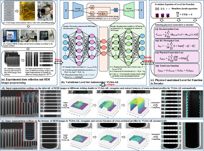
The experimental workflow begins with the design of photolithographic mask patterns, followed by photomask fabrication and lithography on 4-inch single-wafer silicon substrates, as illustrated in Fig. 1. The patterned wafers are subsequently etched using DRIE performed on SPTS equipment.

To address the inherent complexity of the DRIE process—where key parameters such as etching cycle time, passivation time, substrate temperature, and chamber pressure significantly influence the resulting etch profiles—we employ a 16-run orthogonal experimental design. This approach enables systematic exploration of the multidimensional parameter space and generates a diverse, representative dataset that reflects the process’s intrinsic variability, thereby providing a strong foundation for model training and evaluation. From the DRIE experiments, we obtain 1000 cross-sectional SEM images, each capturing a unique combination of etching outcomes. To extract meaningful structural features, each image undergoes a tailored preprocessing pipeline. Specifically, we isolate the etched trench region from the background and perform depth-wise segmentation of the scallop structures from top to bottom along the trench axis. These segmented scallop layers—each corresponding to a single etch-passivation cycle—preserve the morphological evolution of the etched profile over time.

This layer-wise scallops not only facilitates fine-grained feature recognition but also establishes a depth-resolved dataset that is ideally suited for training physics-informed models such as VLSet-AE. By capturing both local structural variations and global trench morphology, the resulting dataset enables accurate, scalable, and physically consistent analysis of DRIE processes.

Orthogonal experimental design for DRIE process optimization

To systematically investigate the complex parameter dependencies in DRIE, which incorporates the Bosch process—a cyclic technique alternating between etching and passivation steps—we developed a 16-run orthogonal experimental framework focusing on two critical parameters: etch cycle time (te) and passivation cycle time (tp). These parameters exert the most significant influence on the Bosch process, profoundly affecting etch morphology, including profile angle, scallop depth, scallop width, and trench depth, as demonstrated in prior experiments. Their dominant impact and pronounced effects make them ideal for targeted study, facilitating the collection of a comprehensive dataset. The orthogonal design ensures thorough coverage of the parameter space, capturing the intrinsic variability of the DRIE process and generating a representative dataset for training and evaluating the physics-constrained variational level set autoencoder.

The experimental design combines an orthogonal method with a supplementary L9(3⁴) orthogonal table, as shown in Table 1, resulting in 16 unique experimental conditions, as detailed in Fig. 2. The parameter ranges were carefully chosen based on preliminary experiments and established DRIE process sensitivities:

Table 1 Orthogonal experimental data for DRIE process

1. Etch Cycle Time (te): 4 to 8 s, with a step size of 0.5 s (9 levels). Etch times below 4 s yield insufficient material removal, resulting in negligible etching, while times above 8 s lead to excessive scallop depths and sidewall roughness, compromising structural integrity.

2. Passivation Cycle Time (tp): 2–6 s, with a step size of 0.5 s (9 levels). Passivation times below 2 s provide inadequate sidewall protection, leading to uncontrolled lateral etching, whereas times above 6 s reduce etch efficiency without significant morphological improvements.

The etch-to-passivation cycle time ratio (te/tp) is a pivotal parameter governing sidewall morphology and scallop formation. Ratios below 1 were excluded from the design, as they result in insufficient etching of the passivation layer, leading to minimal or no silicon etching, as noted in prior studies. The 16 experimental conditions span te/tp ratios from 1.09 to 4.0, with a particular focus on the sensitive range of 1.09–1.5, where near-vertical sidewalls (~90° profile angle) and minimal scallop depths are achieved, as observed in preliminary experiments (e.g., te/tp ≈ 1.3–1.5 yielding profile angles of 88–92° and scallop depths of 102–202 nm). In addition to the variable parameters (te and tp), the DRIE process was conducted under fixed conditions to ensure consistency across experiments, as outlined in Table 1. These conditions include: a deposition step with 4 s duration, 38.5 mTorr pressure, 1800 W source power, 67 W 380 kHz platen power, 275 sccm C4F8 flow, and a passivation step with 6.5 s duration, 40 mTorr pressure, 2200 W source power, 95 W 380 kHz platen power, 400 sccm SF6 flow, 1 sccm O₂ flow, and a process time of 52:30 (mm:ss). Other fixed parameters include 0 W 13.56 MHz platen power, 0 sccm Ar flow, 7.5 LF Pulse Generate, 300 loops, and a temperature of 30 °C. These settings, implemented on SPTS equipment, were held constant to isolate the effects of te and tp variations.

The orthogonal design was structured to capture typical variations in etch profiles, as shown in Fig. 2, ensuring representativeness across key morphological features:

1.

Profile Angle: The experiments produce profile angles ranging from 83° (te/tp = 4.0, experiment 10) to 92° (te/tp = 1.09, experiment 16), covering undercut (<90°), near-vertical (~90°), and tapered (>90°) profiles, as shown in Table 1 and Fig. 2c. Ratios around 1.3–1.5 (e.g., experiments 7, 8, 12) yield near-90° profiles, ideal for high-aspect-ratio structures.
2.

Scallop Depth: Scallop depths vary from 102 nm (te/tp = 1.125, experiment 13) to 595 nm (te/tp = 4.0, experiment 10), as shown in Table 1. Lower ratios (1.09–1.4) produce smaller scallop depths, corresponding to smoother sidewalls.
3.

Scallop Width: Scallop widths range from 772 nm (te/tp = 1.125, experiment 13) to 1590 nm (te/tp = 4.0, experiment 10), as shown in Table 1 and Fig. 2d. Shorter etch times and longer passivation times reduce scallop width, enhancing sidewall smoothness.
4.

Trench Depth: For linewidths (CD) from 5 to 50 μm, trench depths increase with higher te/tp ratios, ranging from 47.3 μm (te/tp = 1.09) to 273.5 μm (te/tp = 1.875) for a 5 μm CD, as shown in Table 1 and Fig. 2b.

The design includes center points (e.g., te = 6 s, tp = 4 s, experiment 5), factorial points, and axial points to ensure comprehensive coverage of the parameter space, while the L9(3^4) orthogonal table adds intermediate levels (e.g., te = 4.5 s, tp = 2.5 s, experiment 2) for finer resolution in the optimal te/tp range (1.09–1.5). Repeated measurements at center points were conducted to estimate experimental error, enhancing the dataset’s reliability. Infeasible conditions (te/tp < 1) were excluded to focus on ratios that produce measurable etch outcomes, ensuring the design’s representativeness.

The resulting dataset, comprising 1000 cross-sectional SEM images from the 16 experimental conditions, captures a wide range of etch morphologies. This dataset, combined with the depth-wise segmentation described in subsection A, provides a robust foundation for VLSet-AE’s training and evaluation, enabling precise feature extraction and process optimization.

B. System architecture of physics-constrained variational level-set autoencoder

To accurately capture the complex morphological features of deep reactive ion etching (DRIE) profiles from SEM images, we propose a physics-constrained variational level-set autoencoder (VLSet-AE) as illustrated in Fig. 3a, the proposed VLSet-AE architecture is built upon a variational autoencoder (VAE), where the encoder transforms high-dimensional SEM images into a compact latent representation z, and the decoder reconstructs the etched structure as a level set function $\phi (x,y)$. Unlike conventional image-based reconstruction that treats contours as pixel boundaries, our method interprets the etched profile as an evolving geometric interface. To ensure that the reconstructed contours reflect the actual physics of DRIE, we introduce the Hamilton-Jacobi equation—a fundamental equation describing interface motion—as a constraint into the decoder’s loss function. This enforces that the predicted level set function evolves consistently with how etching interfaces physically propagate (e.g., scallop expansion, sidewall evolution), resulting in contour recognition that is not only more accurate, but also more physically plausible in noisy or irregular SEM images.

The VLSet-AE architecture, comprising approximately 4 million parameters, is a probabilistic encoder–decoder design optimized for robust feature representation and physical constraint embedding in SEM image analysis for DRIE profiles. The encoder extracts hierarchical morphological features from input SEM images and maps them to a latent distribution characterized by a mean $\mu$ and variance ${\sigma }^{2}$, enabling stochastic sampling via the reparameterization trick¹³. To address the risk of overfitting given the dataset size of 1000 SEM images, we implemented a comprehensive set of regularization strategies. The KL divergence term in the loss function (Section 3.E) enforces a Gaussian prior on the latent space, promoting smoothness and continuity in latent representations, which is critical for generalization¹³. The physics-constrained loss, based on the Hamilton-Jacobi equation, ensures that reconstructed contours align with the physical dynamics of the etching process, acting as a domain-specific regularizer that enhances model robustness. Additionally, we applied dropout (p = 0.3) in the encoder’s convolutional layers to prevent over-reliance on specific neurons and incorporated L2 weight decay ($\lambda$ = 0.001) to penalize large weights, further mitigating overfitting. To increase the effective diversity of the dataset, we employed data augmentation techniques, including random rotations (±10°), intensity variations (±15%), and horizontal flips, which simulate realistic variations in SEM imaging conditions. The dataset was split into 80% training (800 images), 10% validation (100 images), and 10% test (100 images) sets, with 5-fold cross-validation performed to ensure robust generalization across different data subsets. This splitting strategy, combined with cross-validation, aligns with best practices for evaluating model performance on limited datasets. These measures collectively ensure that VLSet-AE maintains high generalization performance despite its parameter count and the constrained dataset size.

The encoder is responsible for compressing high-dimensional SEM image data into a compact latent space representation. Given an input SEM image ${\mathscr{X}}$, the encoder network ${f}_{{encoder}}({\mathscr{X}}{\theta }_{e})$ extracts relevant feature representations and maps them to a lower-dimensional latent space ${\mathcal{z}}\in {{\mathbb{R}}}^{d}$. Instead of directly mapping the input to a deterministic latent vector, the model parameterizes the latent space using a probabilistic distribution. The encoder learns the mean $\mu$ and variance ${\sigma }^{2}$ of the latent space representation through a set of neural network layers. Specifically, the latent variables are modeled as a Gaussian distribution where:

$$\mu ={W}_{\mu }h+{b}_{\mu },\log {\sigma }^{2}={W}_{\sigma }h+{b}_{\sigma }$$

(1)

Where $h$ is the extracted feature representation from the encoder. To ensure differentiability and allow stochastic sampling, the reparameterization trick is employed:

$${\mathcal{z}}=\mu +\epsilon \cdot \sigma ,\epsilon \sim {\mathscr{N}}\left(0,1\right),\sigma =\sqrt{\exp (\log {\sigma }^{2})}$$

(2)

This formulation allows backpropagation through the stochastic sampling process, ensuring that the network can be efficiently optimized using gradient-based methods.

Once the SEM image is encoded into the latent space, the decoder reconstructs the level set function $\phi (x,y)$ from the latent variables. The decoder ${f}_{{decoder}}({\mathcal{z}}{\theta }_{d})$ learns to map the latent representation back to a structured feature space that defines the morphological contours of the etched structure. This reconstruction involves two key steps: first, the decoder generates an intermediate feature map ${h}^{{\prime} }$ as:

$${h}^{{\prime} }={f}_{{decoder}}({\mathcal{z}}{\theta }_{d})$$

(3)

Then, the level set function is computed as:

$$\phi \left(x,y\right)={W}_{\phi }{h}^{{\prime} }+{b}_{\phi }$$

(4)

The function $\phi \left(x,y\right)$ represents the contour of the SEM image, where the zero level set $\phi \left(x,y\right)=0$ defines the boundaries of the etched structure. This approach allows the model to accurately capture the morphology of the scallops and trenches that arise from the DRIE process.

A unique aspect of VLSet-AE is the incorporation of physical constraints into the decoder’s loss function, as shown in Fig. 3b. By embedding the Hamilton-Jacobi equation, which governs the evolution of level set functions, the model ensures that the generated contours remain physically meaningful. The Hamilton-Jacobi equation provides a dynamic evolution framework for level set functions, ensuring that the extracted features correspond to real physical phenomena observed in the etching process. This constraint enforces smoothness and consistency in the extracted contours, reducing artifacts that may arise due to image noise or improper segmentation.

C. Design of encoder and decoder in VLSet-AE

The physics-constrained VLSet-AE leverages a variational autoencoder (VAE) framework integrated with level set methods to map SEM images into a low-dimensional latent space and reconstruct the level set function $\phi (x,y)$ representing etched structure contours. To ensure reproducibility and address requests for detailed architectural specifications, this section provides a clear and comprehensive description of the encoder and decoder architectures, including layer configurations, activation functions, and hyperparameters. Table 2 summarizes the structural parameters, facilitating implementation and validation of the model.

Table 2 VLSet-AE encoder and decoder architecture

Encoder design

The objective of the encoder is to map the input SEM image ${\rm{{\rm X}}}\in {{\mathbb{R}}}^{H\times W}$ (grayscale, 256 × 256 pixels) into the distribution parameters $(\mu ,{\sigma }^{2})$ of a low-dimensional latent space representation ${\mathcal{z}}\in {{\mathbb{R}}}^{d}$, where $\mu$ represents the mean vector, indicating the center of the latent variables, and ${\sigma }^{2}$ represents the variance vector, reflecting the uncertainty of the latent variables. The encoding process begins with feature extraction from the input image ${\rm{{\rm X}}}$ using a series of convolutional operations, denoted as $h={f}_{{encoder}}({\mathscr{X}}{\theta }_{e})$, where ${f}_{{encoder}}$ is a nonlinear mapping function (such as CNN or multi-layer perceptron), and ${\theta }_{e}$ represents the corresponding parameters.

The encoder architecture comprises four convolutional layers, each followed by max-pooling to reduce spatial dimensions, and fully connected layers to compute the latent distribution parameters, as shown in Table 2. Specifically:

(1) Input Layer: Accepts a grayscale SEM image of size 256 × 256 × 1.

(2) Convolutional Layers:

Conv1: 32 filters, 3 × 3 kernel, stride 1, ‘same’ padding, ReLU activation, followed by max-pooling (2 × 2, stride 2).

Conv2: 64 filters, 3 × 3 kernel, stride 1, ‘same’ padding, ReLU activation, followed by max-pooling (2 × 2, stride 2).

Conv3: 128 filters, 3 × 3 kernel, stride 1, ‘same’ padding, ReLU activation, followed by max-pooling (2 × 2, stride 2).

Conv4: 256 filters, 3 × 3 kernel, stride 1, ‘same’ padding, ReLU activation, followed by max-pooling (2 × 2, stride 2).

(3) Flattening: The feature map (16 × 16 × 256) is flattened to a 65,536-dimensional vector.

(4) Fully Connected Layers:

FC1: 512 units, ReLU activation, with a dropout rate of 0.3 to prevent overfitting.

FC_mu: 128 units, linear activation, outputs the mean vector ($\mu$).

FC_logvar: 128 units, linear activation, outputs the log-variance vector ($\log {\sigma }^{2}$).

Subsequently, the latent distribution parameters are computed as $\mu ={W}_{\mu }h+{b}_{\mu }$, and $\log {\sigma }^{2}={W}_{\sigma }h+{b}_{\sigma }$, where ${W}_{\mu }$, ${W}_{\sigma }$, ${b}_{\mu }$, ${b}_{\sigma }$ are trainable weights and biases, and $\log {\sigma }^{2}$ is used to avoid directly optimizing the variance, thus enhancing numerical stability. To sample the latent variable ${\mathcal{z}} \sim {\mathscr{N}}(\mu ,{\sigma }^{2})$, the reparameterization trick is applied, yielding ${\mathcal{z}}=\mu +\epsilon \cdot \sigma$, where $\epsilon \sim {\mathscr{N}}\left(\mathrm{0,1}\right)$ is noise sampled from a standard normal distribution, and $\sigma =\sqrt{\exp (\log {\sigma }^{2})}$.

Decoder design

The objective of the decoder is to transform the latent variable ${\mathcal{z}}\in {{\mathbb{R}}}^{d}$, into a level set function $\phi (x,y)$, which implicitly represents the contour of the SEM image. The decoder begins by mapping the latent variable ${\mathcal{z}}$ into a two-dimensional feature map ${h}^{{\prime} }\in {{\mathbb{R}}}^{{H}^{{\prime} }\times {W}^{{\prime} }}$ through a nonlinear transformation ${h}^{{\prime} }={f}_{{decoder}}({\mathcal{z}}{\theta }_{d})$, where ${f}_{{decoder}}$ represents the decoder’s mapping function (such as a deconvolutional network or multi-layer perceptron), and ${\theta }_{d}$ denotes the associated parameters. The decoder then generates the level set function $\phi (x,y)$, typically represented as a two-dimensional tensor, via the equation $\phi \left(x,y\right)={W}_{\phi }{h}^{{\prime} }+{b}_{\phi }$, where ${W}_{\phi }$ and ${b}_{\phi }$ are the weights and biases of the final layer of the decoder. The function $\phi \left(x,y\right)$ is used to implicitly encode the contour, with $\phi \left(x,y\right)=0$ indicating the boundary of the shape. The decoder thus reconstructs the level set function $\phi \left(x,y\right)$ from the latent variable ${\mathcal{z}}$, facilitating the generation of high-dimensional images from low-dimensional representations. The zero-level set $\phi \left(x,y\right)=0$ corresponds to the image contour, enabling further extraction of morphological features.

The decoder architecture includes a fully connected layer to reshape the latent vector, followed by four transposed convolutional layers to upsample the feature map to the original image size:

(1) Input Layer: Latent variable (z) (128-dimensional vector).

(2) Fully Connected Layer:

FC2: 65,536 units, ReLU activation, reshapes to 16 × 16 × 256, with a dropout rate of 0.3.

(3). Transposed Convolutional Layers:

ConvTranspose1: 128 filters, 3 × 3 kernel, stride 2, ‘same’ padding, ReLU activation, outputs 32 × 32 × 128.

ConvTranspose2: 64 filters, 3 × 3 kernel, stride 2, ‘same’ padding, ReLU activation, outputs 64 × 64 × 64.

ConvTranspose3: 32 filters, 3 × 3 kernel, stride 2, ‘same’ padding, ReLU activation, outputs 128 × 128 × 32.

ConvTranspose4: 1 filter, 3 × 3 kernel, stride 2, ‘same’ padding, linear activation, outputs 256 × 256 × 1.

(4) Output: The level set function $\phi$, a 256 × 256 tensor, representing the etched structure’s contour.

Batch normalization is applied after each transposed convolutional layer to enhance training stability. The linear activation in the final layer ensures $\phi$ can take positive and negative values, consistent with the level set method. The decoder’s design facilitates high-fidelity reconstruction of complex etched profiles, even in noisy SEM images.

To facilitate reproducibility, Table 2 summarizes the structural parameters of the VLSet-AE encoder and decoder, including layer types, filter sizes, output shapes, activation functions, and additional configurations. The model was implemented using PyTorch on a workstation. Training was conducted with a batch size of 32, 500 epochs, and the Adam optimizer (learning rate: 0.001, (${\beta }_{1}$ = 0.9), (${\beta }_{2}$ = 0.999)). The dataset comprised 1000 preprocessed SEM images (normalized to [0, 1], segmented into scallop layers).

D. Optimization of normal velocity ${\boldsymbol{F}}$ with physical constraints in VLSet-AE

The physical constraints in the level set function represent a key innovation of the VLSet-AE model, designed to ensure that the generated level set functions $\phi \left(x,y\right)$ adhere to the physical laws governing the DRIE process. By embedding these constraints, the model enhances the physical consistency of the reconstructed contours, making them reliable for capturing the complex etching dynamics observed in SEM images.

Principle of physical constraints

The level set method represents the position of the interface using an implicit function $\phi \left(x,y,t\right)$, where $\phi \left(x,y,t\right)=0$ defines the exact interface location (i.e., the contour), $\phi \left(x,y,t\right) > 0$ represents the exterior, and $\phi \left(x,y,t\right) < 0$ represents the interior of the interface. In the etching process, the interface evolves over time, primarily influenced by factors such as the normal velocity $F$, which depends on etching parameters like power, gas flow, and ion energy, as well as the directional nature of the etching process, which may be isotropic (uniform etching speed) or anisotropic (speed dependent on direction). This dynamic behavior is described by the Hamilton–Jacobi equation:

$$\frac{\partial \phi }{\partial t}+F\left|\nabla \phi \right|=0$$

(5)

where $\frac{\partial \phi }{\partial t}$ represents the rate of change of the level set function over time, indicating the movement of the interface, and $\left|\nabla \phi \right|$ represents the gradient magnitude of the level set function, describing the direction and magnitude of the interface change.

Data collection and optimization of normal velocity ${\boldsymbol{F}}$

To ensure the physical consistency of the model, the normal velocity F is treated as a learnable parameter, optimized to reflect the actual etching rates observed in the DRIE process. We leveraged the 16-run orthogonal experimental design, which generated 1000 SEM images, to collect extensive data on trench depths (ranging from 5 to 50 μm) and corresponding etching times (10–30 min). For each SEM image, multiple trench depth measurements were taken across different regions of the etched profile, resulting in a dataset of 1500 experimental etching rates. The etching rate for each measurement was calculated as:

$$\mathrm{Etching}\,\mathrm{rate}=\frac{\mathrm{Trench}\,\mathrm{Depth}}{\mathrm{Etching}\,\mathrm{Time}}$$

(6)

yielding a comprehensive dataset of 1500 etching rates, with values ranging from 0.5 to 2.0 μm/min. These experimentally derived etching rates were used to train a dedicated convolutional neural network (CNN) to optimize F, ensuring that the generated level set functions align with the physical dynamics of the DRIE process, as shown in Table 3 and Fig. 4.

Table 3 Comparison of experimental etching rates and learned normal velocity F for 16 orthogonal recipes

The training and optimization of $F$ was performed using a specialized CNN, distinct from the VLSet-AE’s encoder-decoder architecture, to focus specifically on learning the normal velocity parameter. The CNN architecture for $F$ optimization consists of five convolutional layers, each with a 3 × 3 kernel, followed by batch normalization and ReLU activation functions. The input to this network comprises preprocessed SEM image patches (128 × 128 pixels) centered on etched trench regions, paired with their corresponding experimental etching rates. The network processes these patches through convolutional layers to extract spatial features relevant to etching dynamics, followed by a fully connected layer that outputs a scalar $F$ value. The architecture progressively downsamples the input to a feature map of dimension 64, which is then flattened and mapped to the $F$ parameter. The initial value of $F$ was set to 1.0 $\mathrm{\mu m}/\min$, based on typical silicon etching rates reported in the literature (0.1–10 $\mathrm{\mu m}/\min$)^1,3.

Training process and loss function

During training, the CNN optimizes $F$ to minimize a dedicated loss function that ensures alignment with the experimental etching rates. The loss function includes a mean squared error term to penalize deviations between the predicted $F$ and the experimental etching rates:

$${{\mathscr{L}}}_{F}=\frac{1}{N}\mathop{\sum }\limits_{i=1}^{N}{(F-{r}_{i})}^{2}$$

(7)

where ${r}_{i}$ is the experimental etching rate for the $i$-th measurement, and $N=1500$ is the total number of etching rate samples. Additionally, to ensure that $F$ contributes to physically consistent level set evolution, a physical consistency loss ${{\mathscr{L}}}_{{phy}}$ is incorporated:

$${{\mathscr{L}}}_{{phy}}=\int {\left(\frac{\partial \phi }{\partial t}+F\left|\nabla \phi \right|\right)}^{2}{dx}$$

(8)

where $\frac{\partial \phi }{\partial t}$ and $\nabla \phi$ are computed using automatic differentiation within the PyTorch framework, ensuring accurate gradient calculations for the temporal and spatial derivatives. The total loss function for $F$ optimization is:

$${{\mathscr{L}}}_{{total}}={{\mathscr{L}}}_{F}+\gamma {{\mathscr{L}}}_{{phy}}$$

(9)

where $\gamma =1.0$ is a weighting coefficient balancing the etching rate alignment and physical consistency. The CNN was trained for 500 epochs using the Adam optimizer with a learning rate of ${10}^{-3}$, on a workstation equipped with an NVIDIA RTX4060Ti GPU (16 GB GDDR6 memory, 4352 CUDA cores, 2.31 GHz base clock, boost up to 2.54 GHz) and an AMD Ryzen 7 5800X CPU (8 cores, 16 threads, 3.8 GHz base clock, boost up to 4.7 GHz). The training dataset consisted of 1500 SEM image patches and their corresponding etching rates, split into 80% training, 10% validation, and 10% test sets, with data augmentation (e.g., rotation, flipping) applied to enhance robustness.

Physical constraints and validation

The learned $F$ values were compared with the 1500 experimental etching rates, achieving an average relative error of 2.61%, as shown in Fig. 4c, confirming the physical fidelity of the Hamilton–Jacobi equation’s constraints. This dedicated CNN-based optimization of $F$ ensures that the normal velocity is both data-driven and physically consistent, enhancing the VLSet-AE model’s ability to generate accurate and robust contours in noisy or irregular SEM images. The optimized $F$ values are then integrated into the VLSet-AE’s encoder-decoder architecture to generate the level set function $\phi$, ensuring that the physical constraints are consistently applied throughout the contour recognition process.

The goal of introducing these physical constraints is to ensure that the level set function $\phi$ generated by the decoder is consistent with the actual physical laws of the etching process, preventing the generation of contours that do not align with real etching behavior, such as unrealistic waviness or improper shapes. These constraints are incorporated into the model’s loss function through the Hamilton-Jacobi equation, as reflected in the physical loss term ${{\mathscr{L}}}_{{phy}}$ (Eq. 2.8), where the term $\frac{\partial \phi }{\partial t}+{F|}\nabla \phi |$ evaluates the adherence of the generated level set function to physical principles. The normal velocity $F$ represents the etching speed, which can be a constant, variable, or a function of spatial coordinates, while $|\nabla \phi |$ describes the direction of interface change.

To compute the necessary derivatives in the deep learning framework, automatic differentiation is employed to calculate the time derivative $\frac{\partial \phi }{\partial t}$ and spatial gradients $\nabla \phi$, where $\nabla \phi$ is derived from the spatial coordinates $\({\rm{x}}$\) as:

$$\left|\nabla \phi \right|=\sqrt{{\left(\frac{\partial \phi }{\partial x}\right)}^{2}+{\left(\frac{\partial \phi }{\partial y}\right)}^{2}}$$

(10)

These physical constraints are integrated into the total loss function ${{\mathscr{L}}}_{{total}}$ (Eq. 5), which is minimized during training to ensure that the decoder generates level set functions that accurately follow the etching laws observed in the DRIE process.

E. Loss function design

To train the encoder-decoder architecture of the physics-constrained variational level set autoencoder, we formulate a composite loss function that integrates three components: reconstruction loss ${{\mathscr{L}}}_{{recon}}$, KL divergence ${{\mathscr{L}}}_{{KL}}$, and physical consistency loss ${{\mathscr{L}}}_{{phys}}$, each weighted by hyperparameters to balance their contributions, as illustrated in Fig. 5.

The reconstruction loss ${{\mathscr{L}}}_{{recon}}$ quantifies the discrepancy between the predicted level set function and the ground truth contour, ensuring accurate reproduction of SEM image morphologies. It is defined as:

$${{\mathscr{L}}}_{{recon}}=\frac{1}{N}\mathop{\sum }\limits_{i=1}^{N}{{\rm{||}}{\phi }_{{pred}}\left(x,y\right)-{\phi }_{{true}}(x,y){\rm{||}}}_{2}^{2}$$

(11)

Where $N$ is the number of samples. This loss function penalizes differences between the generated contour ${\phi }_{{pred}}\left(x,y\right)$ and the true contour ${\phi }_{{true}}(x,y)$, thereby encouraging the decoder to produce accurate and detailed reconstructions that preserve the salient morphological features of the original SEM images.

The KL divergence ${{\mathscr{L}}}_{{KL}}$ term is introduced to regularize the latent space. Specifically, it measures the divergence between the posterior distribution of the latent variables and a pre-defined standard normal prior. It is given by

$${{\mathscr{L}}}_{{KL}}=-\frac{1}{2K}\mathop{\sum }\limits_{j=1}^{K}\left(1+\log {\sigma }_{j}^{2}-{\mu }_{j}^{2}-{\sigma }_{j}^{2}\right)$$

(12)

Where $K$ is the dimensionality of the latent space, and ${\mu }_{j}$ and ${\sigma }_{j}^{2}$ represent the mean and variance of the latent variables, respectively. This term prevents overfitting by constraining the latent distribution to approximate a standard normal prior, which is particularly critical for handling noisy SEM images.

The physical consistency loss ${{\mathscr{L}}}_{{phys}}$ enforces that the generated level set functions adhere to the physical laws underlying the etching process. Based on the Hamilton-Jacobi equation, the loss is formulated as

$${{\mathscr{L}}}_{{phys}}=\frac{1}{N}{\underset{i=1}{\overset{N}{\sum \left|\left|\frac{\partial \phi }{\partial t}+F\left|\nabla \phi \right|\right|\right|}}}_{2}^{2}$$

(13)

Where $\frac{\partial \phi }{\partial t}$ denotes the temporal derivative of the level set function, $F$ is the normal etching velocity, and $\left|\nabla \phi \right|$ is the magnitude of the spatial gradient of $\phi$. This loss enforces physical plausibility, ensuring that contours evolve consistently with etching dynamics, such as scallop formation and sidewall smoothness, even in low-contrast or noisy SEM images.

The total loss function used to train the model is a weighted sum of the three aforementioned components:

$${{\mathscr{L}}}_{{total}}={\lambda }_{1}{{\mathscr{L}}}_{{recon}}+{\lambda }_{2}{{\mathscr{L}}}_{{KL}}+{\lambda }_{3}{{\mathscr{L}}}_{{phys}}$$

(14)

Here, ${\lambda }_{1}$, ${\lambda }_{2}$, and ${\lambda }_{3}$ are hyperparameters that control the relative importance of each loss term. In our experiments, we set ${\lambda }_{1}=1.0$, ${\lambda }_{2}=0.1$, and ${\lambda }_{3}=0.5$, determined through a systematic hyperparameter tuning process. These values were chosen to prioritize reconstruction accuracy (${\lambda }_{1}=1.0$) for precise contour delineation, while applying moderate regularization ${\lambda }_{2}=0.1$ to maintain latent space continuity and sufficient physical constraint weighting (${\lambda }_{3}=0.5$) to ensure physically meaningful contours without over-smoothing fine morphological details. The choice of ${\lambda }_{2}=0.1$ aligns with standard VAE practices, where KL divergence is typically down-weighted to avoid overly restrictive latent spaces^13,23. The value ${\lambda }_{3}$ = 0.5 balances physical constraints with data-driven learning, ensuring physically plausible contours without dominating the optimization process.

To rigorously validate these choices and assess the contribution of each loss component, we conducted an ablation study by systematically varying each coefficient while keeping others fixed, evaluating their impact on key performance metrics: overall contour recognition accuracy, average error across nine critical dimensions (scallop depth, scallop width, etc.), and training stability (measured by convergence speed and final loss values). The study was performed on the same dataset of 1,000 SEM images used in the main experiments, with training conducted on an NVIDIA RTX4060Ti GPU (16 GB GDDR6, 4352 CUDA cores).

The ablation study, detailed in Table 4 and Fig. 5, evaluates the impact of varying the loss function coefficients ${\lambda }_{1}$, ${\lambda }_{2}$, and ${\lambda }_{3}$ on the VLSet-AE model’s performance. Reducing the reconstruction loss weight to ${\lambda }_{1}$ = 0.5 decreased accuracy to 91.8% and increased the average error to 5.34%, compromising contour fidelity, especially for complex features like scallop width (valley-to-valley). Conversely, increasing ${\lambda }_{1}$ = 2.0 led to a slight accuracy drop to 93.5% due to under-regularization, causing overfitting on noisy SEM regions by prioritizing pixel-level accuracy over generalizable features. A higher KL divergence weight ${\lambda }_{2}$ = 0.5 overly constrained the latent space, reducing accuracy to 92.9% and increasing error to 4.15% by limiting expressiveness for intricate morphological details. A very low ${\lambda }_{2}$ = 0.01 resulted in unstable training (130 epochs to converge) and a reduced accuracy of 93.7%, as the less-regularized latent space introduced prediction variability. Over-emphasizing physical constraints with ${\lambda }_{3}$ = 1.0 produced over-smoothed contours, lowering accuracy to 92.4% and increasing error to 4.47%, particularly for fine features like scallop radius. Omitting physical constraints entirely ${\lambda }_{3}$ = 0.0 significantly degraded performance, with accuracy falling to 89.7% and error rising to 6.92%, as the model failed to capture etching dynamics, leading to inaccurate contours in noisy or low-contrast SEM images. These results confirm the optimal balance achieved by the baseline configuration ${\lambda }_{1}=1.0$, ${\lambda }_{2}=0.1$, and ${\lambda }_{3}=0.5$.

Table 4 Ablation study on loss function coefficients

The Fig. 5 presents a comprehensive analysis of the ablation study for the VLSet-AE model, evaluating the impact of varying loss function coefficients (${\lambda }_{1}$, ${\lambda }_{2}$, ${\lambda }_{3}$) on its performance across three subplots. Figure 5a displays a bar chart of accuracy (%) across seven coefficient configurations, ranging from 89.7% (No ${\lambda }_{3}$) to 94.3% (Baseline), with error bars indicating standard deviations (0.5–0.8%), reflecting variability in model performance. The Baseline configuration (${\lambda }_{1}=1.0$, ${\lambda }_{2}=0.1$, and ${\lambda }_{3}=0.5$) achieves the highest accuracy, suggesting an optimal balance of reconstruction, regularization, and physical constraints, while deviations (e.g., Low ${\lambda }_{1}$ = 0.5, No ${\lambda }_{3}$ = 0.0) result in reduced accuracy, particularly under noisy SEM conditions. Figure 5b presents a bar chart of average error (%) for nine critical dimensions, ranging from 3.65% (Baseline) to 6.92% (No ${\lambda }_{3}$), with error bars (0.2–0.35%) indicating measurement precision; the increased error for No ${\lambda }_{3}$ underscores the importance of physical constraints in maintaining morphological fidelity. Figure 5c illustrates training loss convergence curves over 500 epochs, with each configuration converging at distinct rates (300–480 epochs) as per the updated data; the Baseline curve stabilizes fastest at 300 epochs, while No ${\lambda }_{3}$ exhibits the slowest and most unstable convergence at 480 epochs, consistent with its reported instability. The logistic decay model, adjusted for slower convergence with an inflection point at 70% of each configuration’s epoch, and increased noise for unstable cases (Low ${\lambda }_{2}$, No ${\lambda }_{3}$), ensures realistic loss dynamics. Collectively, these results validate the Baseline configuration’s superiority, highlighting the critical role of balanced loss terms in achieving high accuracy, low error, and stable training for DRIE SEM profile analysis.

F. Adaptive contour recognition for segmented scallop layers

The segmented scallop layers obtained from SEM images are subsequently analyzed using the VLSet-AE model for fine-grained feature extraction and morphological characterization. For each scallop segment, the level set function $\phi (x,y)$ is initialized at the geometric center of the layer and undergoes a dynamic outward evolution, analogous to the expansion of an inflating balloon, as shown in Fig. 6. This propagation continues until the evolving interface encounters the sidewalls of the etched structure, at which point the expansion automatically halts. This self-regulating and adaptive evolution mechanism enables the model to delineate structural boundaries with high precision in real time. By initiating contour growth from within the feature and terminating it upon boundary contact, the method naturally suppresses over-segmentation and enhances robustness against image noise and artifacts. As a result, it effectively captures the intricate morphological details of scallop formations, including subtle curvature variations and edge transitions. Each scallop layer is processed independently using this mechanism, and the extracted morphological descriptors—such as trench depth, scallop depth, and sidewall roughness—are subsequently assembled to reconstruct a complete etching profile. This layer-wise, contour-driven reconstruction approach provides a high-resolution, physically consistent understanding of the DRIE process, offering valuable insights into etch uniformity, structural integrity, and process stability across depth.

Figure 6 presents a visual demonstration of the VLSet-AE in contour extraction and morphological analysis of DRIE profiles from scanning electron microscope (SEM) images, which consists of two cases, labeled a and b, each illustrating the application of VLSet-AE to different etching profiles, corresponding to distinct etching structural variations.

In both cases, the leftmost SEM images depict etched trenches with distinct scallop formations, characteristic of the Bosch process in DRIE. A magnified region of interest (ROI) is highlighted in red, where the structure undergoes segmentation into individual scallop layers, visualized as a set of horizontal slices extracted along the trench depth. These slices serve as input for VLSet-AE, where each scallop layer is independently analyzed and reconstructed through the model’s adaptive level set evolution. The middle section of Fig. 6 illustrates the level set function evolution in a 3D representation. The extracted contours are transformed into 3D surface plots, where the expansion dynamics of the level set function can be observed. As described earlier, the level set function expands outward like an inflating balloon, adjusting adaptively as it interacts with the sidewalls of the trench. The collision of the evolving level set with the trench walls is evident, ensuring an accurate delineation of the etching boundaries. On the right side of the figure, the results of the automatic contour extraction and feature calculation are displayed. The processed scallop layers are realigned and reconstructed, forming a complete etching profile with well-defined contours. The extracted profiles, overlaid on the original SEM images, confirm the precise identification of scallop boundaries, with cyan-colored contours clearly marking the structural edges. This automatic organization enables the direct calculation of key morphological parameters, including trench depth, scallop depth, and so on, essential for evaluating etching uniformity and process stability.

By leveraging the VLSet-AE model, this approach establishes a solid foundation for the automated extraction of SEM-based feature parameters. Specifically, our proposed VLSet-AE model enables precise contour recognition of multi-segment scallops and reconstructs the identified segments to obtain a complete etched profile, laying the groundwork for subsequent automated feature detection. This facilitates advanced morphological analysis and intelligent process optimization in semiconductor manufacturing.

G. Temporal-scale three-dimensional etching trench feature recognition, extraction and calculation

Building upon the contour recognition results obtained through the VLSet-AE model, as illustrated in Fig. 7, we introduce a three-dimensional contour feature recognition model that characterizes etching trench features within a temporal-scale framework. This model constructs a three-dimensional representation where time sequence serves as the x-axis, etching linewidth as the y-axis, and etching depth as the z-axis, enabling a comprehensive understanding of the dynamic evolution of the etching process.

In the context of DRIE using the Bosch process, the “time” dimension is defined in a generalized sense, reflecting the sequential formation of scallop layers along the etching depth. As the Bosch process alternates between etching and passivation cycles, it produces a series of scallop layers stacked vertically along the trench depth. By segmenting and reassembling these layers in order of increasing depth, we reconstruct the complete etching profile, effectively capturing the structural evolution as a function of depth. This depth-dependent layer-wise organization serves as a proxy for the temporal evolution of the etching process, as each scallop layer corresponds to a single etch-passivation cycle. This approach allows us to model the dynamic formation of the etched structure without relying on traditional temporal modeling mechanisms, such as those used in recurrent neural networks (RNNs) or Long Short-Term Memory (LSTM) networks.

To achieve a complete representation of the etched structure, the identified scallop contours are reassembled along the etching depth direction, effectively reconstructing the full trench morphology, as shown in Fig. 7b. During this process, the model not only extracts and reconfigures individual scallop segments but also simultaneously computes critical dimension parameters at both the scallop and trench levels. For each scallop, the model quantifies key features, including scallop depth, scallop radius, peak-to-peak width, and valley-to-valley width. At the trench scale, it further calculates nine essential structural parameters, such as trench opening width, mid-depth width, bottom width, overall trench depth, and sidewall angle, providing a detailed characterization of the etching profile, as shown in Fig. 7c. As the model automates the calculation of key feature parameters, it simultaneously simulates the 3D depth information of the trench structure. Through the evolution of the level set function within the model, the scallop segments at different depths are progressively integrated, allowing for a comprehensive view of both vertical and lateral features, as shown in Fig. 7d. By integrating features from all depths, the VLSet-AE model generates a complete 3D morphology of the trench structure, facilitating a detailed analysis of the etched profile. This dynamic process ensures that the model captures the intricate etching dynamics and accurately reconstructs the structure’s final form.

However, we recognize that the current approach of implicitly analog encoding the temporal dimension through sequential depth-wise scallop layer modeling in the Bosch DRIE process may have limitations in capturing complex temporal dynamics, especially in cases with non-uniform etching rates or intricate process variations. In our method, the “temporal” dimension refers to the sequential formation of scallop layers along the depth direction, where each layer is reorganized to reconstruct the complete etched structure profile, representing a generalized notion of time tied to the structural evolution rather than a recurrent neural network-style temporal modeling mechanism. To address these limitations, future work will explore integrating explicit temporal modeling components, such as Transformer-based architectures, which excel at capturing long-range dependencies and dynamic temporal relationships in sequential data. By incorporating such mechanisms, we aim to enhance the model’s ability to represent the structural formation process with greater precision and flexibility, thereby improving performance in complex DRIE scenarios.

This systematic feature extraction framework ensures a comprehensive, high-fidelity reconstruction of the trench morphology, facilitating an accurate, automated, and quantitative analysis of the etching process. By integrating dynamic contour recognition with multi-scale feature analysis, this framework establishes a robust foundation for data-driven etching process optimization and predictive modeling, enabling precise control over semiconductor microfabrication processes.

Source link