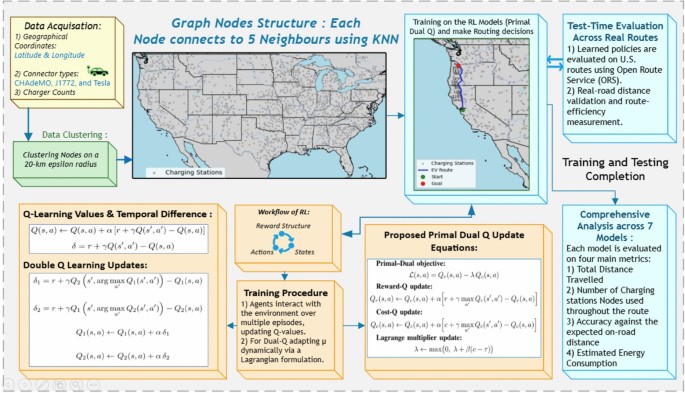
This section details the implementations of training and testing of Reinforcement Learning models (Primal-Dual Q, Q-Learning and Double Q-Learning), standard and improvised versions of A* and Dijkstra which are used to plan routes for Electric Vehicles. The Overall flow of the work is shown in Figure 1.
Data acquisition and graph construction
A nation-wide catalogue of public charging stations was obtained from Alternative Fuels Data Center. Each record provides us with the Latitude of the charging stations (\(\phi\)), Longitude of the charging station (\(\lambda\)), the available Connector types in the charging station (e.g., J1772, CCS-2, CHAdeMO) and the Number of ports available at the charging station \(p\). For graph construction and RL training, the Haversine distance is used to compute edge weights, providing a fast, consistent approximation suitable for large-scale spatial graphs and high-frequency environment interactions during training. For evaluation and final route validation, real-world driving distances are obtained using OpenRouteService (ORS)24, ensuring accurate comparison to actual road-network distances. All maps presented in the figures were generated using the Cartopy library25 with base map data from Natural Earth26. The Graph Construction is done with the help of Latitudes (\(\phi\)) and Longitudes (\(\lambda\)) of the Charging stations. To reduce the graph density, stations are clustered with an \(\varepsilon\)-ball radius of 20 km, i.e., two stations \(i\) and \(j\) become part of the same node if
$$\begin{aligned}&a = \sin ^2\left( \frac{\phi _i – \phi _j}{2} \right) + \cos (\phi _i)\cos (\phi _j)\sin ^2\left( \frac{\lambda _i – \lambda _j}{2} \right) \end{aligned}$$
(1)
$$\begin{aligned}&d(i,j) = 2 R_\oplus \cdot \arcsin \left( \sqrt{a} \right) \end{aligned}$$
(2)

The Learning Process followed by the RL models. Maps generated using Cartopy v0.24.125 with Natural Earth map data26.
The epsilon parameter for DBSCAN was set to 20 km to balance spatial clustering and network connectivity. Smaller epsilon values may produce fragmented clusters that reduce connectivity between charging stations, while larger values may over-aggregate stations and reduce spatial resolution in the routing environment. The selected value provided a practical compromise that preserved connectivity across the large geographic region while maintaining realistic charging station spacing. The Haversine distance between two stations \(i\) and \(j\) is computed using Equations (1) and (2), where \(R_\oplus\) denotes the Earth’s radius (6371 km), and \(\phi\), \(\lambda\) are the latitudes and longitudes in radians. Each node \(v_i \in V\) represents a charging station with a geographic position \(\textbf{x}_i = (\phi _i, \lambda _i)\), where \(\phi\) and \(\lambda\) denote latitude and longitude, respectively. To construct the graph, we connect each node to its \(k\) nearest neighbors using geodesic (Haversine) distance as the metric.The set of \(k\)-nearest neighbors for node \(v_i\) is defined in Equation (3)
$$\begin{aligned} \mathcal {N}_k(v_i)&= \underset{v_j \in V \setminus \{v_i\}}{\operatorname {argmin}^{k}} \; d(v_i, v_j) \end{aligned}$$
(3)
To model both spatial proximity and the utility of charging capacity, the edge weight \(w_{ij}\) between nodes \(v_i\) and \(v_j\) is computed in Equation (4)
$$\begin{aligned} w_{ij}&= \frac{d(v_i, v_j)}{1 + c_j} \end{aligned}$$
(4)
where \(d(v_i, v_j)\) is the geodesic distance between \(v_i\) and \(v_j\), and \(c_j\) is the number of available chargers at node \(v_j\).
The resulting edge set \(E\) is constructed in Equation (5)
$$\begin{aligned} E&= \left\{ (v_i, v_j, w_{ij}) \;\bigg |\; v_j \in \mathcal {N}_k(v_i) \right\} \end{aligned}$$
(5)
This approach creates a charger-aware KNN graph, prioritizing nearby stations with greater charging availability .After clustering and 5-nearest-neighbor construction, the resulting nationwide graph contains approximately 2076 representative charging-station nodes. So with the graph constructed and the proposed RL, classical algorithms learn are trained and tested to find the most optimal path from the start to the destination locations.
Implementations of reinforcement learning models: primal-dual Q learning, Q-learning & double Q-learning
The implementation of the proposed Primal–Dual Q model requires a well-defined EV routing environment, a reward structure that reflects range, charging, and distance constraints, and sufficient interaction for the agent to learn effective policies. The primal–dual formulation introduces an adaptive Lagrangian weighting that balances reward and cost during training, enabling flexible and interpretable control of routing behavior. For completeness, standard Q-Learning and Double Q-Learning models are also implemented within the same environment, following their respective update mechanisms, and serve as baseline reinforcement learning approaches for comparison.
Environment description
We design a custom reinforcement learning (RL) environment for electric vehicle (EV) route planning on a spatial graph. The agent’s goal is to navigate from a given start node to a goal node while optimizing travel efficiency and charging utility. The environment is defined over a graph \(G = (V, E)\), where each node \(v \in V\) has a geographic position and may include metadata such as charger availability and supported connector types. An episode starts at a designated start node and terminates when the agent reaches the goal node. At each timestep, the agent selects an action corresponding to moving to a neighboring node. The environment returns the new state, a scalar reward, and a boolean indicating whether the goal has been reached.
Problem formulation
Formally, the EV routing task is modeled as a constrained Markov decision process (CMDP), where states correspond to graph nodes and actions correspond to transitions to neighboring nodes. The objective is to learn a policy that maximizes cumulative routing reward while limiting cumulative travel cost. This can be expressed as the constrained optimization problem:
$$\begin{aligned} \max _{\pi } \; \mathbb {E}_{\pi }\!\left[ \sum _{t=0}^{T}\gamma ^t R(s_t,a_t)\right] \quad \text {s.t.} \quad \mathbb {E}_{\pi }\!\left[ \sum _{t=0}^{T}\gamma ^t C(s_t,a_t)\right] \le \tau \end{aligned}$$
(6)
where \(R(s_t,a_t)\) denotes the routing reward and \(C(s_t,a_t)\) represents the travel cost. The proposed Primal–Dual Q-learning approach approximates this objective using a dual variable \(\mu\), which adaptively balances reward and cost during learning.
Reward function description
As shown in Table 2, the Reward function is setup such that it would prefer routes with less distance travelled, prefer nodes with necessary connector type of the electric vehicle and avoid detours and delays as much as possible.
Learning algorithm of primal-dual Q-learning
Reinforcement Learning models work upon their experience and hence need training for exploration and exploit the best actions to get maximum rewards. As shown in Algorithm 1, the proposed Primal–Dual Q-Learning with Adaptive Weighting model maintains two distinct value functions: a reward-based Q-table \(Q_r(s,a)\) and a cost-based Q-table \(Q_c(s,a)\). The agent selects actions using a Lagrangian-combined score that balances efficiency against constraint violations. The balance is controlled by a dual variable \(\mu\), which is updated through gradient-based dual ascent. For all reinforcement learning experiments, a learning rate of \(\alpha = 0.1\), a discount factor of \(\gamma = 0.9\), and an \(\epsilon\)-greedy exploration strategy with \(\epsilon\) value being 0.2 is used.
During each transition from state \(s\) to \(s’\) via action \(a\), the reward and cost components are updated using separate temporal-difference (TD) targets. The combined Lagrangian score used for action selection is given in Equation (7). The primal updates for reward and cost values follow Equations (8) and (9), while the dual update rule for \(\mu\), enforcing the cost constraint, is given in Equation (10).
$$\begin{aligned} & \mathcal {L}(s,a) = Q_r(s,a) – \mu \, Q_c(s,a) \end{aligned}$$
(7)
$$\begin{aligned} & Q_r(s,a) \leftarrow Q_r(s,a) + \alpha \Big [ r + \gamma \max _{a’} Q_r(s’,a’) – Q_r(s,a) \Big ] \end{aligned}$$
(8)
$$\begin{aligned} & Q_c(s,a) \leftarrow Q_c(s,a) + \alpha \Big [ c + \gamma \max _{a’} Q_c(s’,a’) – Q_c(s,a) \Big ] \end{aligned}$$
(9)
The dual variable \(\mu\) adjusts according to the magnitude of constraint violation \((c – \tau )\), where \(\tau\) is the target cost threshold:
$$\begin{aligned} \mu \leftarrow \max \Big ( 0,\, \mu + \eta (c – \tau ) \Big ) \end{aligned}$$
(10)
This update corresponds to a dual-ascent step commonly used in primal–dual optimization methods, where the dual variable increases when the cost constraint is violated and decreases when the constraint is satisfied. This primal–dual structure allows the agent to dynamically learn trade-offs between route efficiency and constraint satisfaction (e.g., SoC safety margin, energy cost, or charging availability), producing interpretable and constraint-aware routing policies.
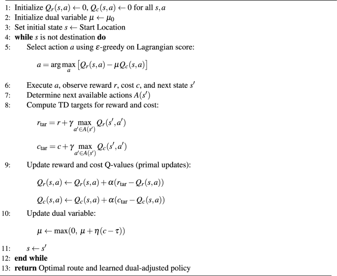
Primal-Dual Q Learning with Adaptive Weighting RL Algorithm.
Learning algorithm of Q and double Q learning
As shown in Algorithm 2, the Learning Algorithm of Q-Learning model only uses a single agent for selecting and evaluating the actions. During the training of the Q-Learning Model, the Q-value is updated using the temporal difference(TD) learning rule. Specifically, when the agent transitions from state \(s\) to a new state \(s’\) by taking action \(a\) and receiving reward \(r\), and then selects a next action \(a’\), the Q-value is updated using the Equation (11). The Temporal difference is calculated using Equation (12).
$$\begin{aligned} & Q(s, a) \leftarrow Q(s, a) + \alpha \left[ r + \gamma Q(s’, a’) – Q(s, a) \right] \end{aligned}$$
(11)
$$\begin{aligned} & \delta = r + \gamma Q(s’, a’) – Q(s, a) \end{aligned}$$
(12)
In Equation (12), \(\alpha\) is the learning rate and \(\gamma\) is the discount factor. The use of \(Q(s’, a’)\) rather than \(\max _{a’} Q(s’, a’)\) indicates that this implementation aligns with the SARSA (on-policy) algorithm than with standard Q-learning (off-policy). As training progresses, the Q-values become optimal under suitable conditions, enabling the agent to act optimally in the environment Fig. 2.
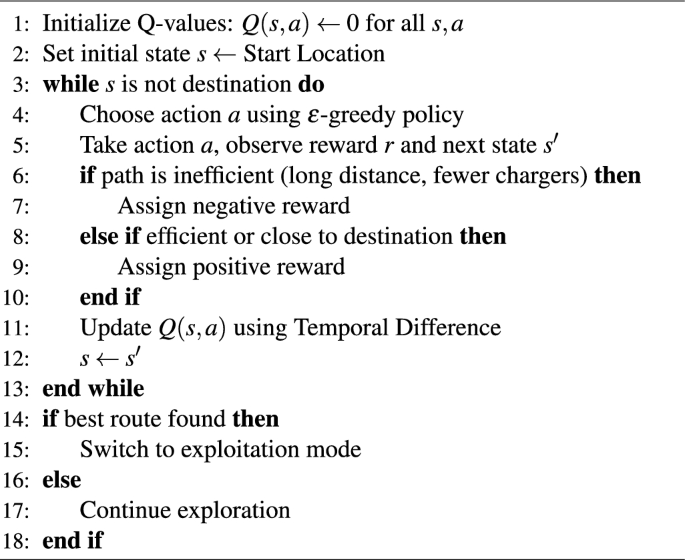
Reinforcement Learning-Based EV Routing Algorithm.

The Learning Process followed by the RL models.
The Learning Algorithm of Double Q-Learning involves two agents. This is because an overestimation in values occurs in Q-Learning model when the same set of Q-values are used for selecting and evaluating actions. To overcome this, Double Q-Learning model uses two sets of Q-values, \(Q_1(s, a)\) and \(Q_2(s, a)\), and decouples the action selection from action evaluation during the learning process. The Temporal differences for 2 set of values is calculated in Equations (13) and (14). The agent chooses actions using an \(\epsilon\)-greedy policy based on the average of the two sets of Q-values and updates one set of values for selection and the other for evaluation as given in Equations (15) and (16).
$$\begin{aligned} & \delta _1 = r + \gamma Q_2\left( s’, \arg \max _{a’} Q_1(s’, a’)\right) – Q_1(s, a) \end{aligned}$$
(13)
$$\begin{aligned} & \delta _2 = r + \gamma Q_1\left( s’, \arg \max _{a’} Q_2(s’, a’)\right) – Q_2(s, a) \end{aligned}$$
(14)
$$\begin{aligned} & Q_1(s, a) \leftarrow Q_1(s, a) + \alpha \, \delta _1 \end{aligned}$$
(15)
$$\begin{aligned} & Q_2(s, a) \leftarrow Q_2(s, a) + \alpha \, \delta _2 \end{aligned}$$
(16)

Overall Process Flow of EV Route Finding using RL Models. Maps generated using Cartopy v0.24.125 with Natural Earth map data26.
Figure 3 illustrates the workflow of the RL-based routing models. The agent learns to find optimal routes on the graph structure by updating Q-values based on observed states and actions until the destination is reached. The graph is first constructed using a K-nearest neighbor (KNN) approach, after which the model learns routing policies through the defined reward system. To improve real-world feasibility, an additional distance-based optimization step is applied by selecting charging nodes within a range of 175–250 km. The initial route generated by the reinforcement learning agent represents node-to-node traversal across the charging station graph. Because stations are connected using a KNN structure, the learned route may include intermediate nodes with shorter distances. Therefore, a filtering stage is applied to skip unnecessary intermediate nodes and enforce realistic charging intervals (175–250 km). In rare cases, shorter segments may still occur when the network topology or charging station availability does not permit a feasible node within the preferred range. This range reflects practical EV operation, where drivers typically utilize only a portion of the nominal 300–400 km vehicle range to maintain a safety margin under real-world conditions.
Implementations of improvised A* and Dijkstra models
Improvised A* Algorithm
The A* search algorithm is one of the traditional models used in routing systems to figure out efficient routes. Here, we use an evaluation function defined in Equation (17) to determine the most promising node to explore next.
$$\begin{aligned} f(n) = g(n) + h(n) \end{aligned}$$
(17)
where f(n) is the total estimated cost of the cheapest solution through node n, g(n) is the known cost from the start node to the current node n, h(n) is the heuristic estimate of the cost from node n to the goal node.
As shown in Algorithm 3, the Improvised A* algorithm adapts the standard A* framework for electric vehicle routing. While it retains the core principle of combining travel cost and heuristic estimates, it introduces EV-specific constraints such as limited battery range by preventing transitions to neighboring nodes if the required distance exceeds the available battery capacity. Additionally, as shown in Equation (18), charging is allowed only at nodes where charging stations are available. This ensures that the generated routes satisfy electric vehicle operational constraints and remain feasible for practical navigation Fig. 4.
$$\begin{aligned} & f(n, b) = g(n) + h(n) \quad \text {subject to } d(n, n’) \le b \end{aligned}$$
(18)
$$\begin{aligned} & b’ = {\left\{ \begin{array}{ll} B_{\text {max}}, & \text {if node } n’ \text { has a charger} \\ b – d(n, n’), & \text {otherwise} \end{array}\right. } \end{aligned}$$
(19)
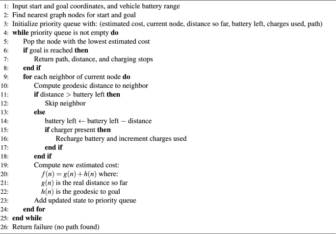
Improvised A* Algorithm for EV Routing

Improvised A* Algorithm Learning Process.
Improvised Djikstra algorithm
Dijkstra’s algorithm is employed to compute the path between two nodes in a graph, using edge weights that represent travel cost, typically distance. The algorithm explores paths in increasing order of cumulative cost from the source using Equation (20).
$$\begin{aligned} f(n) = g(n) \end{aligned}$$
(20)
The Improvised Dijkstra algorithm extends the standard Dijkstra framework by incorporating electric-vehicle constraints such as battery range and charging availability. Unlike the original version, it tracks the vehicle’s current battery level and the number of charging stops. Each state in the priority queue includes the current node, remaining battery, distance traveled, and charges used. When a node has a charging station, the battery is reset and the charge count increases. Edge costs use real geodesic distances between node coordinates. The update rule for computing the shortest distance between consecutive nodes is given in Equation (21).
$$\begin{aligned} d(v) = d(u) + \text {dist}(u, v), \quad \text {only if } \text {dist}(u, v) \le B_u \end{aligned}$$
(21)