Accurate surgery time prediction (ASTP) strategy based on artificial intelligence techniques

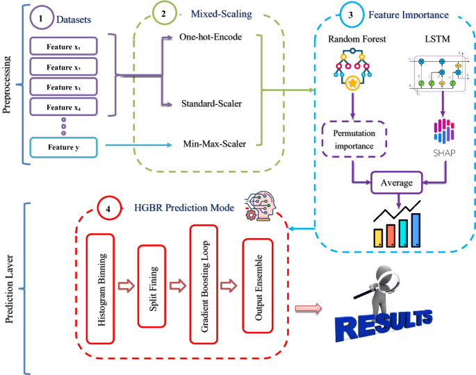
Our strategy consists of two layers as illustrated in Fig. 1. The preprocessing layer performs Mixed-Scaling, computes feature importance using LSTM and Random Forest, and Feature ranking, which orders the features and selects the most informative subset. The prediction layer applies HGBR to the ranked features, yielding the final time-to-surgery prediction.

Preprocessing layer in ASTP

In this layer, the data is processed using One Hot encoding, Mixed-Scaling, and determining the importance and ranking of features.

One hot encoding

In tabular data modeling, each categorical value in Eq. 1 is represented by a one-hot vector of length K (i.e., a \(\:\times\:\) K), where K is the number of possible classes for that categories²⁰. The vector contains zeros in all cells except one with the value 1, which specifies the actual class.

\(\:c=\{\:{c}_{1},\dots\:\dots\:.,{c}_{k}\}\) Is the category set (with size K), x \(\:\epsilon\) c is observed category, \(\:{\left[{\varnothing}\:\right(x\left)\right]}_{k}\:\)denotes the K-th coordinate of the one-hot vector, 1{⋅} is the indicator function (1 if the condition holds, 0 otherwise), n is the number of samples, the one hot block is O \(\:\epsilon\) \(\:{\left\{\text{0,1}\right\}}^{n\times\:k}\) in Eq. 2.

This formulation ensures that the learning model does not assume that “larger numbers are more important,” because simple numerical notations (e.g., “stable = 1, more stable = 2, unstable = 3”) might imply an unreal rank relationship or distance between classes. For example, the value “emerging” is not “more important” than “scheduled” because we write it as 2 instead of 1; they are simply different labels for two classes that should be separated without an imaginary order. In practice, we keep the columns of one-hot values as binary (0/1) without resizing scaling.

Mixed-Scaling

To ensure numerical stability during model training while preserving the semantic meaning of categorical indicators, a mixed-scaling preprocessing strategy is adopted. In this approach, different types of variables are treated according to their statistical characteristics, as illustrated in Fig. 2. The mixed-scaling strategy applies standardization to continuous input features and min–max normalization to the regression target, while leaving the binary/one-hot indicators unchanged. For continuous input features, Z-score standardization is applied. For each continuous feature\(\:{\:X}_{j}\), the mean \(\:{\mu\:}_{j}\) and stander deviation \(\:{\sigma\:}_{j}\:\)on the training split only, and transform every sample \(\:i\) as in Eq. 3.

This centers on features (mean\(\:\cong\:0\)) and scales their variance (\(\:\cong\:1\)), improving numerical stability for gradient-based optimization. Binary and one-hot features remain in {0, 1} without scaling to preserve their presence/absence semantics. Min–Max normalization is applied to the target variable (surgery runtime in minutes). During LSTM training, the target \(\:y\)(runtime in minutes) is mapped to the range [0, 1] using the minimum \(\:{y}_{min}\) and maximum \(\:{y}_{max}\:\)values computed from the training data in Eq. 4:

This scaling stabilizes the optimization process and ensures that the loss function operates within a consistent range. After inference, the predicted values are inverse-transformed to minutes for reporting and interpretation. In the Random Forest pipeline, the target is left in minutes, tree-based ensemble models do not require scaling of the target variable.

Experiencing The Impact of The Ranking/Importance Related to each Feature

At this stage, we employ two models—a single-layer long short-term memory (LSTM) network and a random forest to balance expressive power with robustness on tabular data. The LSTM acts as a gated feature mixer, even with a single time step, capturing subtle nonlinear interactions while maintaining stable gradients through its cell and hidden states with a tanh nonlinearity. A compact dense head maps the LSTM representation to the scalar target. In contrast, the random forest provides a strong, noise-tolerant baseline that requires minimal preprocessing, naturally handles mixed numeric/one-hot inputs, and affords straightforward interpretation via permutation importance. We use both learners as a combined robustness check: their complementary inductive biases probe the same signal from different angles. Agreement between their attributions SHAP for the LSTM and permutation importance (MAE) for the random forest strengthens confidence in the learned relationships, whereas discrepancies highlight features or regimes that merit closer inspection. Where appropriate, a simple averaging ensemble can further reduce variance and improve MAE. In Algorithm 1, the steps of the feature importance (RF permutation and LSTM–SHAP) used to quantify surgical-time drivers are provided.

Long Short-Term Memory (LSTM)

Recurrent neural networks (RNNs) designed to learn long-term temporal dependencies in sequential data. Traditional RNNs struggle to retain information over long time periods because gradients either disappear or explode during backpropagation²¹. LSTM networks address this problem by adding an explicit memory cell and a set of gates that regulate the flow of information, allowing for a stable distribution of values over longer time periods. An LSTM processes a sequence step by step while maintaining two internal states: a cell state \(\:{c}_{t}\)that carries long-term information, and a hidden state \(\:{h}_{t}\) that provides the current output. Three gates (input, forget, and output) control writing, erasing, and reading from the cell. The gates are parameterized by sigmoid (values in [0, 1]) so the model can learn how much new information to admit, how much past information to keep, and how much of the updated memory to expose. A hyperbolic tangent (tanh) nonlinearity proposes new content for the cell and squashes the exposed state, keeping activations bounded and gradients more stable.

In Fig. 3. Show LSTM component used in our model. The LSTM operates on tabular inputs reshaped to a single time step (N, 1, d) maintaining a cell state \(\:{c}_{t}\:\)and a hidden state \(\:{h}_{t}\) while three sigmoid gates (input, forget, output) regulate writing, retention, and exposure of information. The tanh nonlinearity proposes new content and bounds activations, stabilizing gradients; with sequence length one, the forget gate plays a minor role, whereas the input and output gates act as a sample-specific soft mask over the feature-driven proposal. We use a single-layer LSTM (u\(\:\:\in\:\left\{\text{96,128}\right\},tanh\)) followed by dropout (p ∈ {0.10, 0.20}) and a compact dense head (m \(\:\:\in\:\){32, 64}, ReLU), ending with a linear output (Dense (1)) that produces a scalar estimate of time. The target is min–max scaled on the training split and predictions are inverted back to minutes for reporting. After training the LSTM model, SHAP is applied on the validation set to explain how each input feature contributes to the predicted surgical duration. For each validation sample, SHAP assigns an additional contribution value to every feature. These SHAP values are then rescaled by the target range so that the contribution of each feature is expressed directly in minutes. Finally, the overall significance of each feature is calculated as the average of the absolute SHAP value across all validation samples²².

Random forest

Random forests are ensembles of decision trees trained on resampled data, with attribute subsamples taken at each split to separate the trees and reduce variance²³. For an input x, the forest expectation is the mean of the T trees in Eq. 5.

Where \(\:{f}_{t}\) is the prediction of tree\(\:\:t\), In Random forests the output is reported directly in minutes (no target scaling) such as lstm.

Therefore, in parallel, a random forest model is trained on the same input variables, and the importance of its features is estimated using the permutation importance. In this method, the values of one feature are randomly rearranged while keeping the other features unchanged, and the resulting rise in the mean absolute error is recorded as ΔMAE. A larger positive value for ΔMAE indicates that the feature is more influential. Two techniques methods are used together to verify the robustness of the results. If both methods produce a similar ranking, confidence in the feature ranking is strengthened. If differences emerge, this indicates that some variables may behave differently under linear and nonlinear interactions, thus requiring further investigation. The final ranked feature list is used in the next stage, where the HGBR model is evaluated using the TOP-K strategy. Therefore, only the LSTM+SHAP model is used for feature ranking.

Prediction layer in ASTP

In the prediction layer, the features are listed in the order they were taken in the previous Feature Importance and Feature Ranking stage, and we use Histogram Gradient Boosting Regression for prediction. Histogram Gradient Boosting Regression (HGBR) is a gradient-boosted decision tree model that speeds up partition searches by quantizing continuous features across a fixed number of bins and evaluating partitions at bin boundaries rather than all unique values²⁴.

This histogram approximation significantly reduces memory consumption and computational costs while preserving the expressiveness of boosted trees. On structured (tabular) data, HGBR typically achieves high accuracy by capturing nonlinear and feature interactions with minimal feature engineering and without strict input scaling forecasting. The HGBR follows a four-stage mechanism. (1) Histogram binning: continuous features are quantized into a fixed number of bins learned during training. This turns split evaluation from sample-level scans into bin-level scans, improving cache locality and runtime while retaining the expressiveness of boosted trees. (2) Split finding: for each node, prefix-sum scans over the per-bin (and per-feature) aggregated gradients identify the threshold that maximizes loss reduction (gain). (3) Gradient boosting loop: shallow regression trees are fitted to the negative gradients (pseudo-residuals) and added with shrinkage; we use L1 loss with leaf-value smoothing (L2) and early stopping for regularization. (4) Output ensemble: multiple seed models are averaged in log space at inference time (equivalent to a geometric mean on the original scale), yielding a stable predictor. In our pipeline, this module generates log-space predictions that are inverted to minutes for reporting.

In our strategy, we use the Histogram Gradient Boosting Regression (HGBR) model as the main tabular updater to predict the surgical duration (in minutes). The target variable is expressed in minutes and, on the training split only, we apply target preprocessing Winsorization using an IQR rule constrained by the 1st/99th percentiles, followed by log1p transform with an optional non-negative shift s \(\:\ge\:0\). At inference, predictions are mapped back to minutes via Eq. 6.

And all metrics are reported in minutes. We use a priority-ordered feature set from feature ranking stage. The HGBR configuration is tuned for the tabular performance, specifying the loss learning rate, maximum product, maximum leaf nodes, minimum leaf samples, l2 normalization, and maximum bins, with an early internal stop (validation rate = 0.20). Mechanistically, HGBR speeds up boosting by quantizing each feature into up to B bins (we use B \(\:\le\:\) 162) and evaluating split candidates at bin boundaries using bin-level prefix-sum statistics; at each round a shallow tree is fitted to the pseudo-residuals and added with shrinkage. For stability, we train three seed models and average predictions in log space (geometric mean on the original scale). This design yields a fast, robust, and accurate baseline for structured surgical-time forecasting. All steps of Algorithm 2 are explained. Figure 4 illustrate the complete flowchart of the proposed strategy.

Evaluation and results

This section presents the experimental evaluation of the proposed ASTP framework, including the results obtained in each layer and their application to the surgical dataset. The experiments were performed on Windows 11 using the Python programming language. The main libraries used were NumPy, Pandas, SHAP, keras, and Scikit-Learn. The computing environment consisted of an Intel Core i7 processor with 16 GB RAM. Figure 5 illustrates the overall workflow of the proposed Accurate Surgery Time Prediction (ASTP) with all comparisons, which is divided into two layers: Layer 1 for feature ranking and TOP-K extraction, and Layer 2 for model training, evaluation, and reporting.

Dataset

The experiments were applied on two datasets. The first was the Operating room dataset from Nile Hospital²⁵, while the second was The Medical Informatics Operating Room Vitals and Events Repository (MOVER) dataset²⁸.

Operating room data from Nile Hospital

Dataset that contains all surgical operations for the period between December 1, 2023, and December 31, 2023. It consists of seven columns that provide daily information as follows: (1) day, (2) priority, (3) time, (4) patient case, (5) number of staff, (6) dr_age, and (7) family number. The Staff column represents the number of medical staff in the operating room, excluding surgeons, and the Patient Condition column indicates the stability of the patient’s condition and ensures readiness to enter the operating room. The priority column expresses emergency cases and their priority in performing surgery. The dataset contains 471 samples and seven columns. Samples from the modified dataset are shown in Table 2.

The raw data cannot be used directly for prediction because the input variables are represented in heterogeneous formats, including categorical labels, textual time expressions, and numerical values. Therefore, a preprocessing step is required to convert the raw data into a suitable numerical representation for model development. This step converts the date column to a number representing a day during the workweek or weekend, where 0 represents a weekend day and 1 represents a day during the workweek. The patient status column is converted to a number representing steady state with 1 and unstable state with 0. The time column is converted to minutes and scaled using Min-Max, while the feature columns, family number, number of staff and priority are scaled using StandardScaler. Table 3 provides a transformed representation of the dataset after preprocessing. However, in the final ASTP framework, preprocessing is applied in a model-specific manner. Target scaling is used only in the LSTM branch, whereas HGBR and Random Forest operate directly on the target in minutes after their respective preprocessing steps.

MOVER dataset

The Medical Informatics Operating Room Vitals and Events Repository (MOVER) is a perioperative dataset containing structured electronic health records and operating room information for surgical cases. In this study, the dataset used contained 39,381 samples. After preprocessing and feature engineering, the dataset was represented using 14 columns, including 13 input features and one target output, which was surgery_duration_min. Input variables included: sex, primary_anes_type_nm, asa_rating, patient_class_nm, height_cm, weight_kg, bmi, surgery_weekday, surgery_month, scheduled_hour, admit_to_or_hours, procedure_grp, and dx_grp. Several variables were extracted from the original dataset, such as height_cm, weight_kg, bmi, surgery_weekday, surgery_month, scheduled_hour, and admit_to_or_hours, while high-cardinality variables were grouped into procedure_grp and dx_grp. Thus, the final modified dataset used in this work contained 39,381 samples with 13 predictive features and one target variable.

Experimental setup

The principal experimental settings and model parameters adopted in our strategy are consolidated in Table 4. The table summarizes the data partitioning strategy, preprocessing procedures, model-specific hyperparameters, training configuration, and evaluation metrics used throughout the ASTP framework.

The ASTP framework was evaluated using a fixed training-testing split for each dataset, where 70% of the cases were used for training and 30% were reserved for final testing. Therefore, all final performance results reported in the following subsections correspond to unseen real cases that were not used during model development.

Performance metrics

The performance metrics used are (1) mean absolute error (MAE), (2) root mean square error (RMSE), and (3) coefficient of determination (R²), which are calculated to evaluate the prediction accuracy of the dataset for surgical time estimation.

Mean absolute error

MAE is a widely used assessment metric that assesses the average magnitude of errors between predicted values.\(\:\:{\widehat{y}}_{i}\) And the actual observed values \(\:{y}_{i}\) without contemplating their destination. It gives an understandable measure of the average distance between forecasts and true values, given in the same unit as the target variable.

Where n total number of observed,\(\:\:{y}_{i}\) is actual value, \(\:\widehat{y}\:\:\)Is predicted value, and \(\:\left|{y}_{i}-\right.\left.{\widehat{y}}_{i}\right|\) is absolute error for observation \(\:i\).

Root Mean Square Error

RMSE calculates the square root of the average squared difference between the expected values.\(\:\widehat{y}\:\)And the actual observed values \(\:{y}_{i}\). Unlike MAE, RMSE penalizes greater error more severely owing to squaring, making it susceptible to outliers.

Where n total number of observed,\(\:\:{y}_{i}\) is actual value, and \(\:\widehat{y}\:\:\)Is predicted value.

Coefficient of Determination

R² calculates the fraction of variation in real values \(\:{y}_{i}.\) this is explained by the projected values. \(\:{\widehat{y}}_{i}\) It indicates the model’s quality of fit.

.

Where \(\:\:{y}_{i}\)is actual value, \(\:\widehat{y}\:\:\)Is predicted value, and \(\:{\stackrel{-}{y}}_{i}\)mean of actual values.

Feature importance and Ranking on Nile Hospital dataset

The current subsection presents the feature-importance analysis obtained using the two proposed method, LSTM+SHAP and Random Forest permutation importance on the dataset.

Evaluating The Performance of LSTM Along with Applying SHAP for Explanation

In this section, we describe the implementation of LSTM with Explainable AI (XAI) using SHAP to calculate feature importance in the dataset. The goal is to determine the impact of each feature on the output (time of surgical operations) and assess their relative importance. Figure 6 illustrates the significance of SHAP-based features for the LSTM model. The distribution of SHAP values indicates that priority is the most influential feature, followed by family_number and dr_age. Number of staff and patient_case have less influence, while day shows the weakest overall effect. This ranking confirms that the predicted surgical time is depends primarily on information related to priority and procedure.

Table 5 shows the ranking of feature importance based on SHAP values using the mean absolute SHAP value. Higher values indicate the feature’s importance in the model’s decision-making process. Thus, in the mean absolute SHAP value, the priority feature has the highest value, with the features ranked as follows: (priority, Family number, dr_age, number of staff, patient case, and day).

Evaluating the performance of randomforest with applying permutation importance for explanation

In the Random Forest branch, feature importance is measured using permutation importance. Each feature is randomly while the remaining features are kept unchanged, and the corresponding increase in MAE is recorded as ΔMAE=MAE_permuted −MAE_baseline. Larger positive ΔMAE values indicate greater feature importance, while values close to zero indicate limited predictive contribution.

The importance of the permutations was calculated using a cross-validation split of a modified random forest. The mean baseline error (MAE) was 7.35 min. For each feature, we calculated the mean ΔMAE across repeated shuffling. Table 6 illustrate the Permutation importance results in terms of ΔMAE.

Figure 7 confirms the same ranking trend obtained from SHAP. Priority and family_number cause the largest increase in error after permutation, followed by dr_age and number of staff, while patient_case and day contribute only marginally. This suggests that the day variable adds little predictive information to the current dataset.

The LSTM with SHAP Implementation and Random Forest with Permutation Importance provided the same results in terms of the importance ranking of the features, but if the results differed, the prediction system would not be able to know the order of features to input into the model. Therefore, the metrics from the two methods were averaged to produce a single metric that was fed into the temporal prediction system. Table 7 displays the results for the average values.

In the Fig. 8, the average results for mean_abs_shap and ΔMAE are shown. Were the results show that priority (approximately 3.45, or about 37%) has the most impact; changing/disabling it makes the biggest difference in predicted operation time. family_number (approximately 2.78, or about 30%) is the second most important variable. dr_age (approximately 1.81, or about 19%) and number of staff (approximately 0.95, or about 10%) has a medium impact. Patient (approximately 0.22, or about 2%) has a weak impact. day (approximately 0.06, or less than 1%) has negligible impact.

Ablation study to reduce features in the proposed ASTP framework on nile hospital dataset

To further emphasize the importance of the feature selection phase in the proposed ASTP framework, an analytical study was conducted using the HGBR model in two cases: (i) input of all six available features, (ii) input of the top five ranked features, and (iii) input of the top four ranked features, derived from the combined LSTM+SHAP and Random Forest permutation-importance analysis. The ranking results from both methods were highly consistent, with priority, family_number, dr_age, and number of staff identified as the most influential features. The ablation results show that the reduced model with four features achieved a lower mean absolute error (MAE) (8.8857 min) than the complete model with six features (9.0512 min), indicating improved feature efficiency and more accurate predictive representation. On the other hand, the five- and six-feature configurations maintained slightly better root mean square error (RMSE) and R² values than the four-feature configuration, indicating a trade-off between minimizing input dimensions and preserving overall variance fit. Overall, these results confirm the effectiveness of the feature-ranking and TOP- K stages in the ASTP algorithm are effective for minimizing input space while maintaining competitive predictive performance. Table 8 summarizes the effect of feature reduction on the final prediction phase of HGBR.

In-depth evaluation of the HGBR strategy to assess performance effectiveness on nile hospital dataset

From the previous layer, we obtained the following attribute order (priority, family_number, dr_ age, number of staff, patient_case, and day). We apply the model to a set of TOP K, where each K feature is added in the order we obtained from the previous layer. For example, TOP K 1 represents the set consisting of only the priority feature, while TOP K 2 represents the set consisting of priority and family_number. This continues with the remaining sets until TOP K 6, which contains all the features. Table 9 summarizes the prediction performance of the HGBR, ANN, LSTM, GRU, and LSTM + GRU hybrid models across increasing subsets of the TOP-K features. Overall, the HGBR model achieved the lowest mean absolute error (MAE) using the top four ranked features, while the ANN model performed best using all six features. The iterative models (LSTM, GRU, and the hybrid) consistently produced higher errors than the HGBR model across the evaluated subsets. These results suggest that the prediction layer based on the HGBR model is better suited to the current scheduled surgery time dataset.

Table 9 presents the best values achieved by HGBR, ANN, LSTM, GRU, and hybrid(LSTM + GRU). HGBR performed the best, reaching its lowest error with only four features. LSTM, GRU, and hybrid (LSTM + GRU) achieved their lowest values with two features; however, these values were still higher than those of HGBR. As the number of features increased, the values continued to rise, while ANN performed better than LSTM, GRU, and hybrid (LSTM + GRU), but with six features, as illustrated in Fig. 9.

The ASTP framework was evaluated as an integrated pipeline on a 30% reserved test subset. The best overall performance was achieved by the HGBR-based ASTP configuration using the top four ranked features, resulting in a mean absolute error (MAE) of 8.89 min, a root mean square error (RMSE) of 19.5 min, and a coefficient of determination (R²) of 0.26. This indicates that on average, final expectancy of ASTP differs from the actual surgery duration by approximately 8.89 min in real, non-visualized test cases. Figures 10 and 11, and 12 show a comparison of the best performance of each model across different metrics, demonstrating that HGBR outperforms the other systems.

Statistical Significance Analysis on Nile Hospital dataset

To assess whether the observed differences between the comparative models were statistically significant, a non-parametric statistical analysis of the absolute prediction errors was performed on the same reserved test set. Specifically, a pair-permutation test was applied, and a 95% Bootstrap confidence interval was calculated for the mean absolute error difference (MAE). The MAE difference was defined as:

ΔMAE = MAE _HGBR – MAE _{compared model}.

where a negative value indicates that HGBR achieved a lower prediction error than the comparative model.

In Table 11 statistical significance analysis confirmed that the HGBR-based ASTP model significantly outperformed all comparable models. Compared to the Artificial Neural Network (ANN), the mean absolute error (MAE) difference was − 1.1049 min, with a p-value of 0.0084 and a 95% confidence interval (CI) of −1.9152 to −0.2889. Compared to the LSTM, the MAE difference was − 2.8140 min, with a p-value of 0.0001 and a 95% CI of −3.6093 to −2.0243. Compared to the GRU, the MAE difference was − 2.8516 min, with a p-value of 0.0001 and a 95% CI of −3.7002 to −2.0308. In comparison with the LSTM + GRU hybrid model, the mean absolute error (MAE) difference was − 3.1327 min, with a p-value of 0.0001 and a 95% confidence interval ranging from − 3.9444 to −2.3302. Since all p-values were less than 0.05 and none of the confidence intervals include zero, the superiority of the HGBR model is statistically significant. These results provide formal statistical evidence that the reduction in prediction error achieved by HGBR is not due to random variance in the test subset, but reflects a consistent predictive advantage of the current structured surgical time dataset.

From the results shown in Table 10 and the statistical significance analysis in Table 11, HGBR provided the best results in the previous comparison, so it was compared with other research works.

Evaluation on the MOVER Dataset

Table 12 presents the prediction performance of the HGBR, ANN, LSTM, GRU, and LSTM + GRU models across increasing TOP-K ranked feature subsets on the MOVER dataset. The results show that the HGBR model consistently achieved the strongest performance in most TOP-K settings. As the number of ranked features increased from TOP-1 to TOP-7, the HGBR model exhibited a steady decrease in prediction error, with the mean absolute error (MAE) decreasing from 88.64 min at TOP-1 to 77.70 min at TOP-7, accompanied by corresponding improvements in the root mean squared error (RMSE) and the coefficient of determination (R²). This trend indicates that the proposed ranking strategy was effective in ranking the most informative features, and that the incremental addition of higher-ranking variables improved the predictive performance of the models.

Among the neural network-based models, the Artificial Neural Network (ANN) model achieved the best overall performance, with its lowest error at TOP-4, a mean absolute error (MAE) of 81.20, a root mean square error (RMSE) of 120.65, and a coefficient of determination (R²) of 0.2287. However, its performance did not stabilize when additional ranked features were added, indicating that the ANN model benefited from a limited subset of informative inputs but was less robust than the HGBR model in handling the full ranked feature progression. Similarly, the GRU model performed best at TOP-6, while the LSTM + GRU hybrid model performed best at TOP-7. Despite these improvements, both models remained inferior to the HGBR model in terms of overall prediction accuracy. The LSTM model showed the weakest overall performance among the models, recording relatively high prediction errors and low or even negative R² values in many TOP-K settings. In contrast, the superior performance of the HGBR model confirms that tree-based boosting methods are more suitable for this type of structured perioperative data, where nonlinear interactions can be effectively observed without the need for sequential time modeling.

The results show that the HGBR model is best suited for predicting surgical duration on the MOVER dataset within the evaluated TOP-K subsets. Although the best numerical performance of the HGBR algorithm was achieved at TOP-12, the improvement beyond TOP-7 was minimal. Therefore, TOP-7 was selected as the preferred compact predictive subset, as it provides a good balance between prediction accuracy and input complexity. These results support the effectiveness of the proposed feature ranking mechanism and the suitability of the HGBR model as the final prediction model within the ASTP framework.

Figure 13 illustrates the mean absolute error (MAE) performance of the HGBR, ANN, LSTM, GRU, and LSTM + GRU models across increasing TOP-K ranked feature subsets on the MOVER dataset. The results show that the HGBR model achieved the most stable behavior and the lowest overall prediction error, while the other models exhibited greater variability as additional features were included.

To achieve a balanced comparison between predictive performance and feature utilization efficiency, Table 13 presents the best numerical result and best subset for each evaluated model on the MOVER dataset, in terms of mean absolute error (MAE), root mean square error (RMSE), and coefficient of determination (R²). This presentation highlights not only the absolute best performance achieved by each model but also the most practically efficient operating point in terms of reducing input dimensions. In particular, this allows for a more accurate interpretation of the HGBR-based ASTP framework by distinguishing between its best numerical configuration and its best subset, where only minor differences in accuracy are observed despite the reduced number of selected features.

Comparison with previous studies

Table 14compares the proposed HGBR-based ASTP model with other methods published in previous articles.The proposed HGBR model achieves a mean absolute error (MAE) of 8.89 min, a root mean square error (RMSE) of 19.5 min, and a coefficient of determination (R²) of 0.26 using only four features, demonstrating good predictive performance with reduced input dimensions. Although XGBoost and the basic gradient boosted-tree method achieve better numerical results, they rely on six features and do not provide the same efficiency as ASTP in reducing the number of features. Similarly, RandomForest (General) and RandomForest (Dept-spec) both use six features and offer competitive results, although their predictive errors remain slightly higher than those of XGBoost. These results indicate that the proposed HGBR model provides a competitive and practically efficient solution for predicting surgical time on structured tabular data. In addition to direct model comparisons, a methodological comparison was conducted with similar recent studies published in 2025. Kwong et al¹³. reported strong performance based on artificial neural networks in predicting the duration of common elective general surgical procedures at three academic centers, while Ramamurthy et al¹⁷. demonstrated the importance of integrating machine learning with clinical text representations and later extended this approach using large-scale linguistic models to predict surgical duration. Levin et al²⁶. also confirmed the usefulness of boosted tree models in predicting the duration of surgical procedures in each specialty.

Compared to these recent studies, the proposed ASTP framework is distinguished by its integration of interpretable feature ranking, feature reduction using TOP-K, and efficient HGBR-based prediction using structured and compressed tabular inputs. Therefore, the current framework not only offers competitive predictive performance but also improved feature economy and practical interpretability. Figures 14 and 15, and 16 show a comparison between each metric.

Table 15 illustrates an in-depth comparison of the evaluated models. The HGBR system demonstrates strong overall performance with a mean absolute error (MAE) of 8.89 min, a root mean squared error (RMSE) of 19.5 min, and R² of 0.26, using only four features, making it efficient and low-cost for clinical use. Artificial neural networks (ANNs) achieve the highest R² (0.32) with six features, indicating improved correlation, but at the expense of hyperparameter tuning sensitivity. Both the LSTM-GRU, as well as hybrid LSTM + GRU system, show lower efficiency on surgical data (mean absolute error ≈ 11.7–12.0 min) and require long training times (20–85 s), limiting real-time predictability. With a mean absolute error (MAE) of 8.70 min and a root mean square error (RMSE) of 18.4 min, XGBoost provides somewhat higher accuracy than HGBR; nevertheless, it necessitates the use of all six characteristics and meticulous parameter adjustment. While RandomForest (Dept-spec) offers personalized predictions but necessitates big datasets, RandomForest (General) produces competitive results (MAE = 9.0 min, RMSE ≈ 18.7 min) with extremely quick prediction times, making it appropriate for real-world applications.