A super-resolution framework for downscaling machine learning weather prediction toward 1-km air temperature

Study area

The Korean Peninsula exhibits a unique combination of geographical, topographic, and climatic interactions. Its landscape includes mountains, plains, and coastlines, with a distinct north–south orientation and sharp elevation differences between east and west^31,32. Land use is equally diverse, spanning dense urban centers such as Seoul to rural regions dominated by agriculture and forests^33,34. Surrounded by three seas, the peninsula is shaped by strong land–ocean interactions. It experiences a typical mid-latitude climate with four distinct seasons, marked by large temperature contrasts between summer and winter. These characteristics make the Korean Peninsula an ideal natural laboratory for testing the generalizability of temperature super-resolution models across diverse environmental conditions. Our study area was South Korea, where in situ observational data are available (Supplementary Fig. S2).

Deriving 1 km daily air temperature from MODIS LST

High-resolution daily mean air temperature data are required to enhance the spatial resolution of coarse daily temperature products. However, satellite-derived high-resolution daily mean air temperature products are currently unavailable. Therefore, following Yoo et al.³⁵, we transformed the 1 km MODIS land surface temperature (LST) from the MOD11A1 v061 product into the daily mean air temperature, MODIS AT^36,37. To maximize coverage, we used Terra LST only, combining daytime and nighttime observations from both the previous day and the same day. As auxiliary predictors, we included incoming solar radiation, NDVI, latitude, longitude, digital elevation model (DEM), terrain aspect, and impervious surface fraction. Daily mean air temperatures from Automatic Weather Stations (AWS) served as training targets, whereas data from the Automated Synoptic Observing System (ASOS) were reserved for validation. The model, trained on AWS data and evaluated using ASOS data, achieved an RMSE of 1.22 K and R² of 0.95, substantially outperforming direct MODIS LST-derived means (RMSE = 4.13 K; R² = 0.47). Finally, the model was applied to generate a gridded MODIS AT dataset for 2000–2020.

Data

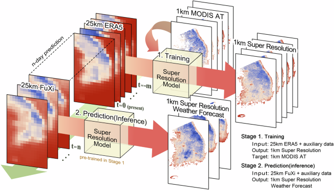
FuXi performs global weather forecasting at a spatial resolution of 0.25° and a temporal resolution of 6 h using an autoregressive architecture with more than 70 surface and upper-air meteorological variables derived from ERA5 reanalysis data collected at 6 h intervals between 1979 and 2017¹⁵. In T2M forecasting, FuXi outperformed conventional numerical weather prediction (NWP) and deep learning models, particularly at extended lead times. WeatherBench 2 provides FuXi T2M forecasts for 2020³⁸. However, using data from a single year (2020) limits the availability of data for model training and validation. In this study, we developed a generalizable super-resolution model for T2M over South Korea based on 0.25° ERA5 T2M data and evaluated its performance using T2M forecasts generated by FuXi. We also used forecasts from KMA’s high-resolution NWP system, LDAPS, as a comparison baseline to evaluate the performance of our model. LDAPS delivers T2M forecasts at approximately 1.5 km spatial resolution and 1-hour temporal resolution over the Korean Peninsula and provides short-range predictions out to 48 h.

A 1 km DEM and Imp data were used as common auxiliary inputs for both training and validation. The DEM was obtained by resampling the 2012 SRTM Void-Filled 3 arc-second dataset to a 1 km resolution³⁹. For Imp, we reconstructed 1 km² grids by calculating the proportion of the urban class within each grid based on the 500 m MODIS Land Cover product (MCD12Q1 v061)^40,41. The MODIS Land Cover product has been available annually since 2001, and for each forecast date, Imp data from the previous year were used as input. For training data from 2000 and 2001, Imp data from 2001 were used. In addition, we propose an SCM to provide seasonally invariant spatial temperature information.

SCM is a spatial temperature map derived from MODIS AT data averaged over 2000 to 2020. It was generated by averaging the temperatures across all years for each calendar day, resulting in 365 average temperature maps corresponding to each day of the year. Because MODIS satellite products frequently contain missing values due to atmospheric conditions such as cloud cover, we applied an 11-day moving average to smooth the data and correct for missing values (Equations (1)–(3)). This procedure also helps reduce potential biases associated with individual days by incorporating temporal context from surrounding dates. Here \({T}_{t,y,i,j}\) denotes the MODIS AT value for the day of year \(t\) (1-365), year \(y\), and spatial coordinates \((i,j)\); \({S}_{t}\) is the result of moving average smoothing; \({B}_{t}\) is the number of years with valid observations on day t (i.e., the number of non-missing values); and \(I({T}_{t,y,i,j})\) is an indicator function that returns 1 if \({T}_{t,y,i,j}\) is valid (i.e., not missing) and 0 otherwise.

To further minimize missing values in the SCM dataset, we implemented an additional interpolation process. Because repeated smoothing over a broad temporal window can obscure day-specific temperature characteristics, an unsmoothed average temperature map \(\hat{T}\) was first derived. This map was then combined with the moving average result \({S}_{t}\) to calculate \({W}_{t}^{\left(n\right)}\) (Equations (4) and (5)): An 11-day moving average was subsequently reapplied to \({W}_{t}^{\left(n\right)}\), and only regions where the number of valid observations in the previous step \(\left({B}_{t}^{\left(n-1\right)}\le 1\right)\) were replaced with the interpolated values (Equations (6) and (7)). In particular, regions where \({B}_{t}^{\left(n-1\right)}\) was one, corresponding to areas influenced by a single observation in the previous moving average step, were updated to mitigate the effects of potential outliers. This update further prevents overreliance on a single observation and improves the robustness of the resulting temperature maps. This iterative process (Equations (5)–(7)) was repeated ten times to produce the final smoothed map, \({S}_{t}^{\left(10\right)}\).

Standard normalization was applied to \({S}_{t}^{\left(10\right)}\) using the mean and standard deviation computed for each calendar day. These statistics were derived from ERA5 data over the entire land area of South Korea for each day of the year (days 1–365). The resulting SCM dataset comprises 365 daily spatial anomaly maps (Supplementary Fig. S3). This dataset represents the relative temperature anomalies within the Korean Peninsula for each calendar day, indicating whether a given location exhibited higher or lower temperatures than other regions during that period. Owing to persistent regional climate patterns, some areas consistently appear warmer or cooler than others during specific seasons.

Air temperature super-resolution using SR-weather

The SR-Weather model in this study was based on the SE-SRCNN proposed by Yasuda et al.²². The SE-SRCNN applies skip connections and a squeeze-and-excitation (SE) block-based channel attention mechanism to extract and integrate features individually from low-resolution temperature data and high-resolution auxiliary data to reconstruct high-resolution temperatures. In SE-SRCNN, the low-resolution temperature input is first resampled using bicubic interpolation to match the spatial resolution of the high-resolution auxiliary data before being fed into the model. The resampled low-resolution and auxiliary data were processed separately through convolutional layers, followed by ReLU activation to extract feature maps. These feature maps were then combined, and the channel attention weights were computed using an SE block. The attention weight for each channel is a scalar value indicating its relative importance. Specifically, global average pooling (GAP) is applied to aggregate spatial information within each channel, producing a single scalar per channel. The aggregated values were passed through two fully connected layers with ReLU and sigmoid activations to compute the attention weights. These weights are then multiplied by the original feature maps, enhancing the contribution of informative channels while suppressing less important ones. The weighted feature maps were subsequently passed through another convolutional layer, and a skip connection was employed to add bicubic-interpolated low-resolution data to the output, producing the final super-resolution temperature field.

In SE-SRCNN, GAP is used to aggregate spatial information for channel attention computation. However, because GAP averages spatial information into a single scalar per channel, it cannot capture distinctive localized features or peaks within feature maps⁴². This averaging bias is particularly problematic when salient signals occupy a small spatial support or appear as sharp gradients. To address this limitation, SR-Weather extends the SE-SRCNN architecture by incorporating global max and min pooling in addition to GAP (Fig. 6). For each pooling operator, we computed channel descriptors and fed them into a lightweight two-layer gating network to obtain separate channel-attention maps, which were then fused to produce the final attention. In the maximum and minimum branches, the gates are conditioned only on DEM and SCM, which biases attention toward topographic and climatological controls. This design increases sensitivity to sharp, localized signals while preserving the global context and improving the reconstruction over high-elevation ridges and valley floors.

Comparison models for air temperature super-resolution

HAT integrates a window-based self-attention architecture from the Swin Transformer family with GAP–based channel attention through a hybrid attention block, enabling the joint learning of local and global information²⁰. The model enhances receptive field coverage by strengthening the information exchange between adjacent windows using an overlapping cross-attention module and convolution-based positional encoding. High-resolution images were reconstructed using a combination of pixel shuffle-based upsampling and subsequent convolutional refinement. HAT demonstrated state-of-the-art performance in the field of single-image super-resolution (SISR) from 2022 to 2023. In this study, HAT was adopted as a comparison model to benchmark performance in the 25× single-image upscaling task, given its demonstrated superiority in this domain.

SRGAN is a representative super-resolution model that employs a generative adversarial network (GAN) architecture to reconstruct perceptually realistic high-resolution images from low-resolution inputs²¹. The generator expands low-dimensional input features into higher-dimensional representations using multiple residual blocks and pixel-shuffle–based upsampling blocks. The discriminator is trained to distinguish between generated and real high-resolution images, thereby providing feedback that encourages the generator to produce outputs that closely match the distribution of natural images. In this study, the SRGAN was configured similarly to the SE-SRCNN, utilizing auxiliary data for super-resolution, to evaluate the applicability of the GAN framework. Because the high-resolution MODIS AT data used in this study contained missing values, partial convolution filters were applied to the discriminator⁴³. This design ensures that missing values do not affect the discriminator’s judgement, allowing the generator to focus on restoring realistic textures rather than predicting the missing data.

Model settings for each model

All variables were scaled to a range of [0, 1]. For both low- and high-resolution temperature data, standard normalization was first applied using the same procedure as for the SCM, followed by [0, 1] normalization. Table 1 summarizes the input variables and corresponding patch sizes used to achieve a 25× spatial resolution enhancement. For the SE-SRCNN and SR-Weather, low-resolution inputs were resampled using bicubic interpolation to match the dimensions of the high-resolution auxiliary data before being input into the model. For all models except HAT, the low-resolution temperature data were divided into 3 × 3 patches with one-third overlap in both directions (stride = 2 pixels). HAT, a SISR model that relies solely on low-resolution temperature data, can suffer degraded performance when trained using excessively small low-resolution patches⁴⁴. Given the limited availability of satellite-based temperature data owing to operational constraints and weather conditions, low-resolution data for HAT were divided into 5×5 patches. Training patches were selected only when the corresponding high-resolution patch contained more than 100 valid pixels, yielding 10,558 training samples for HAT and 39,162 for the other models. During training, pixels without valid MODIS AT observations were masked out from the loss computation to prevent the model from learning from physically unavailable or uncertain target values.

Inference on FuXi forecasts

We trained SR-Weather on ERA5 inputs and applied it to FuXi forecasts, which may have distributions differing from those of ERA5. This approach follows prior DLWP work, which suggests that forecast errors are relatively insensitive to whether the initial conditions come from operational analyses or the ERA5³⁶. To assess the ability to enhance the spatial resolution of forecasts, FuXi 0.25° forecasts from 2020 were provided as inputs to the models trained on the ERA5 0.25° data. The auxiliary data configuration remained identical to that used during training, with 2019 Imp data used to match the latest available land cover conditions before the 2020 forecast period. The input FuXi forecasts were temporally aligned with the target ERA5 data based on forecast initialization and lead times. Daily mean fields from the FuXi model were obtained by averaging the four 6-hourly forecasts within each 24-hour window. Forecast lead times of 1–7 days were evaluated to examine the models’ ability to preserve forecast quality across increasing prediction horizons.

No additional preprocessing was applied to the FuXi inputs beyond standard normalization, which is consistent with the training procedure. To ensure consistency in the evaluation, the models were applied in a patch-based inference mode identical to that used during training. The performance was analyzed separately for each lead times, enabling an assessment of how forecast lead times influence the spatial super-resolution capability of the models.

Evaluation metrics and statistical analysis

Model performance was evaluated using RMSE and R², computed by comparing the super-resolved temperature outputs with the corresponding high-resolution MODIS AT data or in situ observations, depending on data availability. For visual analysis, spatial distributions of RMSE, R², and MBE were calculated for the test period using Equations (8)–(11). These maps, based on the temporal mean values of the super-resolved and reference temperatures (Equation (8)), highlight spatial patterns of model accuracy and systematic bias across the domain. Here, SR denotes the model-predicted high-resolution temperature field, and HR denotes the MODIS AT. D is the set of day-of-year indices for which both SR and HR are valid, \(t\) is the day of the year (1–365), and \((i,j)\) are spatial coordinates.

For a consistent comparison of computational cost, we computed the number of FLOPs per three-dimensional grid cell. Because LDAPS does not publicly disclose FLOPs per time step, we used the WRF CONUS 12-km benchmark as a representative proxy for estimating LDAPS-level complexity. The WRF benchmark reports 22–28.5 × 10⁹ FLOPs per time step for a 433 × 308 × 35 grid, corresponding to 4.7–6.1 × 10³ FLOPs per grid cell per step. With a 1 min integration interval (60 steps per hour), a 36 h LDAPS forecast is therefore approximated to require roughly 1.0–1.3 × 10⁷ FLOPs per grid cell.