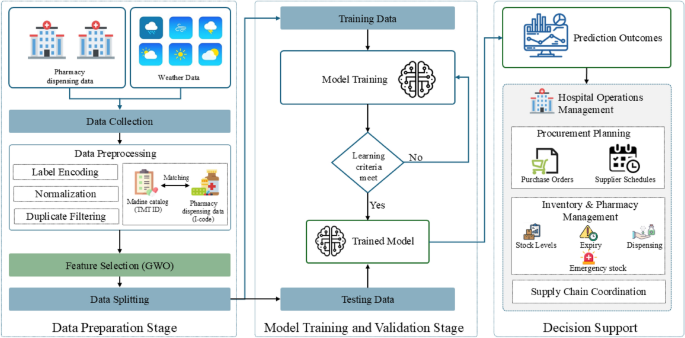
A hybrid grey wolf optimized eXtreme gradient boosting-based machine learning model for hospital pharmaceutical demand forecasting

This study proposes a Hybrid GWO–XGBoost model for hospital-level pharmaceutical demand forecasting. The model integrates real-world hospital dispensing data, standardized drug catalogues, meteorological variables, and temporal features to improve predictive accuracy and model generalization. The overall workflow of the proposed approach is illustrated in Fig. 1, consisting of three main stages: (i) Data Preparation, (ii) Model Optimization and Training, and (iii) Forecast Evaluation. While the conceptual framework highlights possible extensions for hospital decision support, this study focuses primarily on the forecasting and evaluation stages. To assess forecasting performance, the proposed Hybrid GWO–XGBoost model is benchmarked against five baseline machine-learning models and evaluated using three standard performance metrics: Mean Absolute Error (MAE), Root Mean Squared Error (RMSE), and the coefficient of determination ($R^2$).

Study setting and data sources

This study utilized real-world operational data from two provincial hospitals:Pasang Hospital and Banthi Hospital in Lamphun Province, Thailand. The dataset spans from October 2023 to May 2025 and includes over 3.4 million records of outpatient visits, pharmacy dispensing events, and associated service items. Of these, approximately 1.4 million entries were successfully linked to valid Drug Identifier (DID) codes, representing 588 distinct medications, yielding a catalogue match rate of 92.7%. The unmatched records primarily consisted of non-medication items such as laboratory tests, consumables, and service charges, which were excluded from the forecasting analysis to ensure focus on pharmaceutical utilization patterns. Table 2 presents a summary of the integrated dispensing dataset used in this study.

Table 2 Summary of the integrated dispensing dataset used in this study.

Figure 2 presents the distribution of the top 15 dispensed medicines during 2024 across Pasang and Banthi Hospitals, showing substantial variation in consumption levels among different therapeutic categories. This diversity highlights the heterogeneity of medicine demand across time and between hospitals, emphasizing the importance of robust forecasting techniques.

In addition, localized meteorological data were obtained from the Open-Meteo Archive API⁹, covering parameters such as temperature, precipitation, humidity, wind speed, and solar radiation. These variables were synchronized with the hospital datasets according to date and geographic location. Temporal predictors, including the year, month, and week number, were incorporated to represent seasonality and healthcare utilization patterns. These multi-domain datasets were subsequently used to train and evaluate the Hybrid GWO–XGBoost model, enabling assessment of how environmental and temporal factors contribute to variations in hospital medicine demand. Table 3 summarizes the main predictor domains integrated into the forecasting framework.

Table 3 Predictor domains integrated into the forecasting model.

Data preparation and preprocessing

The data preparation process standardized, cleaned, and integrated the multi-source datasets prior to model development. Each hospital’s internal drug catalogue (I-code) was mapped to Thailand’s National Drug Code and the Thai Medicines Terminology (TMT), which is the official standardized terminology for medicines in Thailand, enabling interoperability across hospital information systems. The preprocessing pipeline consisted of the following steps:

Cleaning Removal of duplicate, incomplete, or irrelevant entries (e.g., non-drug service items).
Transformation Log-transformation of weekly demand values, $\log (1 + y)$, to reduce skewness and stabilize variance.
Encoding Categorical variables were one-hot encoded, and continuous variables were standardized to ensure uniform feature scaling.
Integration Weekly aggregation and temporal alignment of dispensing, weather, and time-series variables across hospitals.

Finally, the processed dataset was divided chronologically into training (80%) and testing (20%) subsets to preserve temporal dependencies and reflect real-world forecasting conditions.

Feature selection using grey wolf optimizer (GWO)

Feature selection plays a crucial role in constructing efficient and interpretable predictive models, particularly for complex healthcare datasets that combine hospital dispensing, meteorological, and temporal variables. Selecting redundant or irrelevant predictors can reduce model accuracy and increase computational cost. To address this challenge, this study employs the GWO⁸, a nature-inspired metaheuristic algorithm modeled on the leadership hierarchy and cooperative hunting behavior of grey wolves. GWO has demonstrated strong convergence stability and a good balance between exploration and exploitation, making it suitable for feature selection in nonlinear, high-dimensional healthcare data^28,29.

In the proposed Hybrid GWO–XGBoost model, each wolf search agent represents a candidate binary vector of features, where “1” denotes inclusion and “0” denotes exclusion. The population is initialized randomly and updated iteratively according to the top three wolves–$\alpha$ (best), $\beta$ (second-best), and $\delta$ (third-best)–which guide the others toward the optimal subset.

The encircling mechanism of prey is mathematically expressed as:

$$\begin{aligned} \vec {D}_{\alpha } = |\vec {C}_1 \cdot \vec {X}_{\alpha } – \vec {X}|,\quad \vec {D}_{\beta } = |\vec {C}_2 \cdot \vec {X}_{\beta } – \vec {X}|,\quad \vec {D}_{\delta } = |\vec {C}_3 \cdot \vec {X}_{\delta } – \vec {X}|, \end{aligned}$$

(1)

where $\vec {X}$ is the position vector of a wolf (feature subset), and $\vec {X}_{\alpha }$, $\vec {X}_{\beta }$, and $\vec {X}_{\delta }$ are the positions of the leading wolves. The coefficient vectors $\vec {C}_1$, $\vec {C}_2$, and $\vec {C}_3$ introduce stochastic variations in movement.

The hunting process is defined as:

$$\begin{aligned} \vec {X}_1 = \vec {X}_{\alpha } – \vec {A}_1 \cdot \vec {D}_{\alpha },\quad \vec {X}_2 = \vec {X}_{\beta } – \vec {A}_2 \cdot \vec {D}_{\beta },\quad \vec {X}_3 = \vec {X}_{\delta } – \vec {A}_3 \cdot \vec {D}_{\delta }, \end{aligned}$$

(2)

and the wolves update their positions as:

$$\begin{aligned} \vec {X}(t+1) = \frac{\vec {X}_1 + \vec {X}_2 + \vec {X}_3}{3}. \end{aligned}$$

(3)

The coefficients $\vec {A}$ and $\vec {C}$ controlling exploration and exploitation are defined as:

$$\begin{aligned} \vec {A} = 2\vec {a}\cdot \vec {r}_1 – \vec {a}, \quad \vec {C} = 2\vec {r}_2, \end{aligned}$$

(4)

where $\vec {r}_1$ and $\vec {r}_2$ are random vectors in [0, 1], and $\vec {a}$ decreases linearly from 2 to 0 over the iterations to gradually shift focus from exploration to exploitation.

To perform binary feature selection, the continuous values of $\vec {X}$ are converted into binary inclusion decisions using a sigmoid transfer function:

$$\begin{aligned} F(x) = {\left\{ \begin{array}{ll} 1, & \text {if } \sigma (x) \ge \gamma , \\ 0, & \text {otherwise,} \end{array}\right. } \end{aligned}$$

(5)

where $\sigma (x)$ is the sigmoid activation and $\gamma$ is a random threshold within [0, 1].

The fitness function guiding the optimization is defined as:

$$\begin{aligned} F = w_1 (1 – R^2) + w_2 \frac{|S|}{|S_{total}|}, \end{aligned}$$

(6)

where $R^2$ is the coefficient of determination from the XGBoost predictions, |S| is the number of selected features, and $|S_{total}|$ is the total number of available predictors. The weights $w_1$ and $w_2$ (set to 0.9 and 0.1, respectively) balance forecasting accuracy and model simplicity. Through iterative updates, GWO searches for the subset of features that minimizes F, retaining only the most informative predictors influencing weekly pharmaceutical demand. The optimized subset is then used for XGBoost model training, forming the complete forecasting pipeline.

Model training and validation

Following the feature selection stage, the optimized subset of predictors identified by the GWO was used to train the forecasting model based on the eXtreme Gradient Boosting (XGBoost) algorithm³⁰. XGBoost is a scalable and regularized gradient boosting framework designed to enhance predictive accuracy and prevent overfitting. It is particularly effective for structured healthcare datasets because of its ability to model nonlinear dependencies, handle missing values, and integrate heterogeneous variables.

In the training phase, XGBoost constructs an additive ensemble of regression trees, where each new tree iteratively learns to correct the residuals of previous trees. Given a training dataset $\mathcal {D} = \{(x_i, y_i)\}_{i=1}^{n}$, where $x_i \in \mathbb {R}^m$ represents the selected input features (hospital dispensing, meteorological, and temporal variables) and $y_i \in \mathbb {R}$ denotes the weekly medicine demand, the model prediction $\hat{y}_i$ is expressed as:

$$\begin{aligned} \hat{y}_i = \sum _{k=1}^{K} f_k(x_i), \quad f_k \in \mathcal {F}, \end{aligned}$$

(7)

where $\mathcal {F}$ denotes the functional space of regression trees and K represents the total number of boosting rounds.

The optimization objective combines a convex loss function $\ell (y_i, \hat{y}_i)$, which measures prediction error, with a regularization term $\Omega (f_k)$ that penalizes overly complex trees, thereby improving generalization³⁰:

$$\begin{aligned} \mathcal {L}(\phi ) = \sum _{i=1}^{n} \ell (y_i, \hat{y}_i) + \sum _{k=1}^{K} \Omega (f_k), \end{aligned}$$

(8)

where the regularization term is defined as:

$$\begin{aligned} \Omega (f) = \gamma T + \frac{1}{2}\lambda \Vert w\Vert ^2, \end{aligned}$$

(9)

with T being the number of leaves in the tree, w the leaf weights, $\gamma$ the complexity penalty, and $\lambda$ the L2 regularization parameter. The first term of the objective function enforces predictive fidelity, while the second controls model complexity, effectively mitigating overfitting.

The loss function used in this study was the Mean Squared Error (MSE):

$$\begin{aligned} \ell (y_i, \hat{y}_i) = (y_i – \hat{y}_i)^2, \end{aligned}$$

(10)

which measures the squared difference between observed and predicted demand values. The final model was trained with tuned hyperparameters, including a learning rate of 0.05, a maximum tree depth of 15, 500 boosting rounds, and regularization parameters $\lambda = 1.5$ and $\gamma = 0.2$.

Decision support integration

The final stage conceptually links the forecasting outcomes to hospital operations intelligence (Fig. 1). Forecasted pharmaceutical demand can be translated into actionable insights across key management domains, supporting proactive and data-driven decision-making:

Procurement planning Supports adjustment of purchase orders and supplier schedules to prevent medicine shortages or overstock situations.
Inventory and pharmacy management Enables dynamic stock-level optimization, expiry monitoring, and preparedness for emergency demand surges.
Supply chain coordination Facilitates improved coordination with regional warehouses and the Government Pharmaceutical Organization (GPO) for timely and efficient distribution.

Although the implementation of a decision-support system is beyond the scope of this paper, the proposed Hybrid GWO–XGBoost forecasting framework provides a foundational analytical layer that can be extended to hospital management dashboards. This integration has the potential to strengthen forecasting precision, optimize resource allocation, and enhance the sustainability and resilience of healthcare supply chains.

Baseline methods

To benchmark the performance of the proposed model, several widely used machine learning (ML) algorithms were implemented as baselines. These models were selected for their strong performance in structured data forecasting and healthcare analytics applications.

Decision tree (DT)

Decision Trees are non-parametric models that recursively partition the input space into homogeneous regions³¹. For regression, the prediction in a terminal node $R_m$ is given by:

$$\begin{aligned} \hat{y}(x) = \frac{1}{N_m} \sum _{i \in R_m} y_i, \end{aligned}$$

(11)

where $N_m$ is the number of training samples in $R_m$. In this study, the DT model was tuned using cross-validation, with a maximum depth of 15, yielding the best validation performance.

Random forest (RF)

Random Forests extend decision trees by constructing an ensemble of trees using bootstrap aggregation (bagging) and random feature selection³². The prediction is obtained by averaging across M trees:

$$\begin{aligned} \hat{y}(x) = \frac{1}{M} \sum _{m=1}^{M} f_m(x). \end{aligned}$$

(12)

Hyperparameters were optimized using grid search with cross-validation. The optimal configuration employed 500 trees, a maximum depth of 15, and $\sqrt{p}$ feature selection at each split, where p is the number of predictors.

Light gradient boosting machine (LightGBM)

LightGBM is a gradient boosting framework optimized for efficiency and scalability³³. It uses a histogram-based algorithm and grows trees leaf-wise, selecting the split with the maximum loss reduction. At iteration t, the prediction is expressed as:

$$\begin{aligned} \hat{y}_t(x) = \hat{y}_{t-1}(x) + \eta f_t(x), \quad f_t \in \mathcal {F}, \end{aligned}$$

(13)

where $\eta$ is the learning rate, $f_t$ is the regression tree fitted to the gradient of the loss function at iteration t, and $\mathcal {F}$ denotes the space of regression trees. The final tuned configuration used a learning rate of 0.05, 500 boosting rounds, a maximum depth of 15, and 64 leaves.

CatBoost

CatBoost is a gradient boosting method designed to reduce prediction shift and efficiently handle categorical features³⁴. Unlike traditional boosting, it employs ordered boosting, which builds each new tree using target statistics computed on a permutation of the training data. Formally, the prediction at iteration t is given by:

$$\begin{aligned} \hat{y}_t(x_i) = \hat{y}_{t-1}(x_i) + \eta f_t(x_i \mid \sigma _{

(14)

where $f_t(x_i \mid \sigma _{ denotes the tree trained on permutations \(\sigma _{ that exclude the current sample i, ensuring unbiased estimates of categorical feature statistics. This mechanism mitigates overfitting and enhances generalization. The tuned configuration used a learning rate of 0.05, 500 iterations, and a maximum tree depth of 15.

Artificial neural network (ANN)

Artificial Neural Networks (ANNs) approximate complex nonlinear relationships through layers of interconnected neurons³⁵. They are commonly used in healthcare forecasting due to their ability to model temporal dynamics and nonlinear dependencies in demand data. Each hidden neuron computes a weighted sum of its inputs followed by a nonlinear activation. The Rectified Linear Unit (ReLU) activation was used in hidden layers, while the output layer used a linear activation suitable for regression tasks.

For an input vector \(x \in \mathbb {R}^m$, the transformation at hidden layer l is:

$$\begin{aligned} h^{(l)} = \max \left( 0, \, W^{(l)} h^{(l-1)} + b^{(l)} \right) , \quad l = 1, \dots , L, \end{aligned}$$

(15)

where $W^{(l)}$ and $b^{(l)}$ denote the weight matrix and bias vector of layer l. The final prediction is obtained as:

$$\begin{aligned} \hat{y} = W^{(o)} h^{(L)} + b^{(o)}, \end{aligned}$$

(16)

where $W^{(o)}$ and $b^{(o)}$ are the parameters of the output layer.

Parameter optimization used the Adam optimizer³⁶, which combines momentum and adaptive learning rates. The best ANN architecture contained three hidden layers with 128, 64, and 32 neurons, respectively, each using ReLU activation. Training employed a batch size of 64, a learning rate of 0.001, and 500 epochs.

All baseline models were tuned through grid search with cross-validation, and the configuration achieving the lowest validation error was selected for performance comparison against the proposed model.

Evaluation metrics

Model performance was evaluated using three standard metrics: Mean Absolute Error (MAE), Root Mean Squared Error (RMSE), and the coefficient of determination ($R^2$). These measures jointly assess predictive accuracy, sensitivity to large deviations, and explanatory power.

The Mean Absolute Error (MAE) quantifies the average magnitude of prediction errors, providing an intuitive measure of model accuracy in the same units as the target variable. The Root Mean Squared Error (RMSE) penalizes larger errors more strongly, emphasizing the model’s ability to handle extreme variations in demand. The coefficient of determination ($R^2$) indicates the proportion of variance in observed demand explained by the model, reflecting its overall goodness of fit.

The three evaluation metrics are formally defined in Equations 17 to 19^37,38:

$$\begin{aligned} MAE = \frac{1}{n} \sum _{i=1}^{n} \left| y_i – \hat{y}_i \right| \end{aligned}$$

(17)

$$\begin{aligned} RMSE = \sqrt{ \frac{1}{n} \sum _{i=1}^{n} (y_i – \hat{y}_i)^2 } \end{aligned}$$

(18)

$$\begin{aligned} R^2 = 1 – \frac{ \sum _{i=1}^{n} (y_i – \hat{y}_i)^2 }{ \sum _{i=1}^{n} (y_i – \bar{y})^2 } \end{aligned}$$

(19)

Here, $y_i$ and $\hat{y}_i$ denote the observed and predicted weekly demand, respectively, and $\bar{y}$ represents the mean observed demand. Together, these complementary metrics provide a balanced evaluation of model accuracy, error dispersion, and explanatory strength in pharmaceutical demand forecasting.

Code availability

The code used to develop and evaluate the proposed model is available at DOI: 10.5281/zenodo.19387761.