The study was designed to use a freely available open TB CXR dataset as training data for the AI algorithm. Subsequent accuracy analysis was conducted using an independent CXR dataset and actual TB cases from our hospital. All imaging data was anonymized to protect privacy. The study was reviewed and approved by the Institutional Review Board (IRB) of Kaohsiung Veterans General Hospital and the requirement for informed consent was waived (IRB number: KSVGH23-CT4-13). This study adhered to the principles of the Declaration of Helsinki.
Training Dataset
A flowchart of the study design is shown in Figure 1. Due to the high prevalence of TB and the variable imaging findings, TB cannot be completely ruled out even when CXR shows pneumonia or other pathologies. Preliminary studies showed that training the model only on TB and normals resulted in a bimodal distribution of predictive values. Therefore, CXRs that were abnormal but not suggestive of TB had predictive values that were either too high or too low, and could not effectively distinguish abnormal cases from normal or TB. For common CXR abnormalities such as pneumonia and pleural effusion, the risk of TB is low but not zero. Therefore, we trained two models using two different training datasets, one for TB detection and the other for anomaly detection. We then averaged the output predicted values.
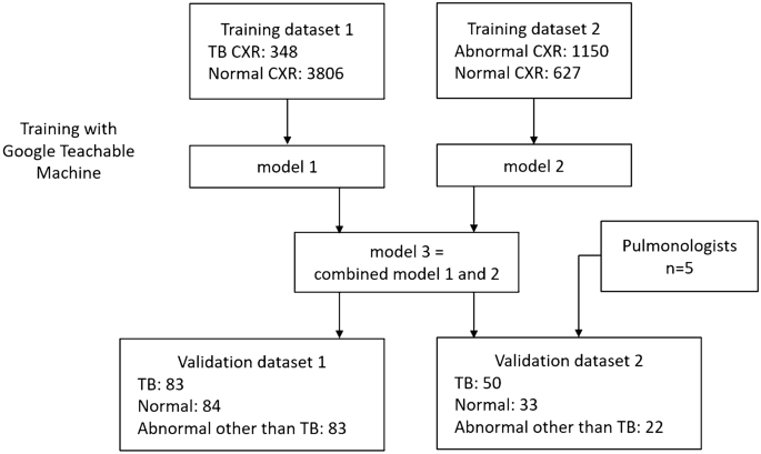
Flowchart for model training and validation.
The characteristics of the training CXR dataset are summarized in Table 1. Inclusion criteria were CXRs with tuberculosis, other abnormalities, or normal. Both anteroposterior and anterior-posterior views were included. Exclusion criteria were poor quality CXRs, lateral view CXRs, pediatric CXRs, and CXRs with lesions too small to be detected at a size of 224 × 224 pixels. All CXR images were reviewed by a CFC to ensure both image quality and accuracy.
Training dataset 1 is used to train the algorithm to detect typical TB patterns on CXRs. For training, 348 TB CXRs and 3806 normal CXRs were collected from various open datasets, including the Shenzhen dataset from Shenzhen Third People's Hospital and the Montgomery dataset.19,20and Kaggle's RSNA Pneumonia Detection Challenge21,22.
Training dataset 2 is used to train the algorithm for detecting CXR abnormalities. A total of 1150 abnormal CXRs and 627 normal CXRs were collected from the ChestX-ray14 dataset.twenty threeAbnormal CXR was: consolidation: 185, cardiomegaly: 235, pulmonary edema: 139, pleural effusion: 230, pulmonary fibrosis: 106, and masses: 255.
Algorithms: Google's trainable machines
GoogleTM was used in this study.18is a free online AI software dedicated to image classification. GoogleTM provides a user-friendly web-based graphical interface that allows users to perform deep neural network computations and train image classification models with minimal coding requirements. By leveraging the power of transfer learning, GoogleTM significantly reduces the computation time and amount of data required to train deep neural networks. Within GoogleTM, the base model for transfer learning was MobileNet, a model pre-trained by Google on the ImageNet dataset containing 14 million images and capable of recognizing 1,000 classes of images. Transfer learning is achieved by modifying the last two layers of the pre-trained MobileNet and maintaining it for subsequent specific image recognition training.18,24In GoogleTM, all images are scaled and cropped to 224 × 224 pixels for training. 85% of the images are automatically split into a training dataset and the remaining 15% into a validation dataset for calculating accuracy.
The hardware used in the study included a 16-core 12th-generation Intel Core i9-12900K CPU running at 3.2-5.2GHz, an NVIDIA RTX A5000 GPU with 24GB of error-correcting code (ECC) graphics memory, 128GB of random access memory (RAM), and a 4TB solid-state disk (SSD).
External validation dataset
To evaluate the accuracy of the algorithm, clinical CXR data of TB, normal cases, and pneumonia/other diseases were collected from our hospital.
Validation dataset 1 included 250 de-identified CXRs collected retrospectively from the VGHKS. The CXR dates ranged from January 1, 2010 to February 27, 2023. The dataset included 83 TB cases (81 microbiology confirmed and 2 pathology confirmed), 84 normal cases, and 83 non-TB abnormal cases (73 pneumonia, 14 pleural effusion, 10 heart failure, and 4 fibrosis; some cases had composite features). The image sizes of these CXRs were: width: 1760-4280 pixels, height: 1931-4280 pixels.
Validation dataset 2 is a smaller dataset derived from validation dataset 1 to compare the performance of the algorithm and physicians, and contains CXRs of 50 TB cases, 33 normal cases, and 22 non-TB abnormal cases (22 pneumonia, 5 pleural effusion, 1 heart failure, and 1 fibrosis). The characteristics of the two validation datasets are shown in Table 1.
Data collected from clinical CXR cases included demographic data (e.g. age and sex), radiological reports, clinical diagnosis, microbiological reports, and pathological reports. All clinical TB cases included in the study had microbiologically or pathologically confirmed diagnoses. CXRs were performed within 1 month of TB diagnosis. Normal CXRs were also reviewed by the CFC and radiological reports were taken into account. Pneumonia/other disease cases were identified by reviewing medical records and laboratory tests and diagnosed by clinical physician judgement, with no evidence of TB detected within 3 months.
Physician Performance Test
We used validation dataset 2 to evaluate the accuracy of TB detection for five clinicians (five board-certified pulmonologists, mean years of experience 10 years, range 5–16 years). Each clinician performed the test without any additional clinical information and was asked to estimate the likelihood of TB in each CXR, consider whether sputum TB testing was necessary, and classify it into three categories: typical TB pattern, normal pattern, and abnormal pattern (not TB-like).
We also collected radiology reports from validation dataset 2 to evaluate the sensitivity for TB detection. Reports mentioning suspected TB or M. tuberculosis infection were classified into typical TB pattern. Reports showing abnormal patterns such as infiltration, opacity, pneumonia, exudate, edema, mass, or tumor (but not mentioning “TB”, “TB”, or “M. tuberculosis infection”) were classified into abnormal pattern (not TB-like). Reports showing no obvious abnormalities were classified into normal pattern. Furthermore, by analyzing pulmonologists' decisions regarding sputum TB testing, we estimate the sensitivity of TB detection in pulmonologists' real clinical practice.
Statistical analysis
Continuous variables are expressed as mean ± standard deviation (SD) or median (interquartile range). [IQR]) and categorical variables are expressed as numbers (percentages). For accuracy analysis, receiver operating characteristic (ROC) curves were used to calculate the area under the curve (AUC). Sensitivity, specificity, positive predictive value (PPV), negative predictive value (NPV), likelihood ratio (LR), overall accuracy, and F1 score were calculated. Confusion matrices were used to demonstrate the accuracy of each AI model. Box plots were used to evaluate the distribution of predicted values of the AI models for each etiology subgroup.
The formula for each precision is as follows:
(TP is true positive, TN is true negative, FP is false positive, FN is false negative, P is all positive, N is all negative.)
$$\begin{gathered} {\text{P}} = {\text{TP}} + {\text{FN}}, \hfill \\ {\text{N}} = {\text{TN}} + {\text{FP}}, \hfill \\ {\text{sensitivity}} = {\text{TP}}/{\text{P}} \times {1}00, \hfill \\ {\text{specificity}} = {\text{TN}}/{\text{N}} \times {1}00, \hfill \\ {\text{PPV}} = {\text{TP}}/\left( {{\text{TP}} + {\text{FP}}} \right) \, \times {1}00, \hfill \\ {\text{NPV}} = {\text{TN}}/\left( {{\text{TN}} + {\text{FN}}} \right) \, \times {1}00, \hfill \\ {\text{LR}} + \, = {\text{sensitivity}}/\left( {{1} – {\text{specificity}}} \right), \hfill \\ {\text{LR}} – \, = \, \left( {{1} – {\text{sensitivity}}} \right)/{\text{specificity}}, \hfill \\ {\text{Overall accuracy}} = \, \left( {{\text{TP}} + {\text{TN}}} \right)/\left( {{\text{P}} + {\text{N}}} \right) \, \times {1}00, \hfill \\ {\text{F1 score}} = \, \left( {{2 } \times {\text{sensitivity}} \times {\text{ PPV}}} \right)/\left( {{\text{sensitivity}} + {\text{ PPV}}} \right) \, \times {1}00, \hfill \\ \end{gathered}$$