A dataset for machine learning model to convective initiation detection and nowcasting over southeastern China

Data source

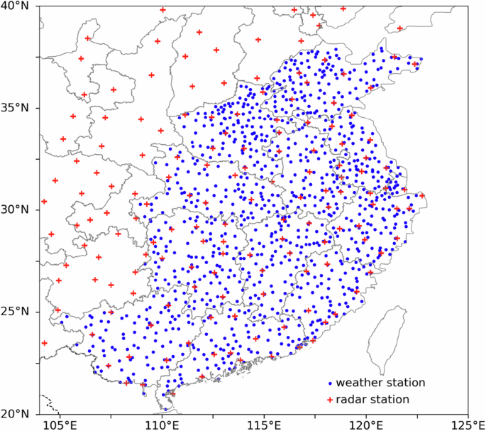
This study uses ground-based meteorological observations to identify severe convective weather events, weather radar data to assign CI labels, and radar and satellite data to characterize features. All data are sourced from the operational database of the National Meteorological Information Center, China Meteorological Administration. CIDS covers the region 104–125°E, 20–40°N (Fig. 1) from March to September, 2018–2023, Southeastern China is dominated by the East Asian monsoon, with the vast majority of severe weather events occurring between March and September. Weather radar and satellite data were sampled within this area. Severe convective weather event samples were drawn from 1,008 national-level surface weather stations of 12 provinces in southeastern China (blue dots in Fig. 1). Event identification used minute-by-minute precipitation, wind speed, and manual hail records from the stations. All data underwent operational quality control. The study area was covered by up to 157 weather radars (122 S-band, 35 C-band). Radar observations underwent quality control to remove non-precipitation echoes, including noise filtering, radial interference recognition, and echo elimination¹⁸. For isolated echo and radial clutter removal, an AI-based electromagnetic interference echo identification method is employed: isolated interference echoes are filtered at the regional level, while radial interference echoes are identified and removed by examining continuity in both radial and azimuth directions. Fuzzy-logic algorithms are used to eliminate terrain, sea-wave clutter, and clear-sky echoes. Concurrently, manual inspection is applied to remove faulty echoes. The radar mosaics method employs the maximum value approach, in which the maximum radar reflectivity value for a given grid cell is assigned a weight of 1, while all other values are assigned a weight of 0. This means the maximum radar reflectivity value for the same grid cell is assigned to it.

Severe convective events sampling

Machine learning training datasets require abundant samples. Given the low probability of severe convective events (SCE) associated with CI, we maximized the number of SCE samples collected. Using minute-by-minute precipitation, wind speed, and hail records from 1,008 stations (March–September, 2018–2023; Fig. 1), we identified periods of heavy precipitation (≥20 mm/60 min), thunderstorm winds (instantaneous wind speed ≥17 m/s with lightning), and hail (hail diameter ≥2 mm). Sample data during SCE periods served as positive CI samples. To include negative samples and accommodate continuous time series for forecasting, the SCE-S period was extended by 2 hours before and 1 hour after the event. This yields single-station severe weather events (SCE-S). From 2018 to 2023, there were 57,252 SCE-S events. After expanding the time window, different SCE-S events at the same station may overlap temporally. Similarly, SCE-S events across different stations within the study area may also overlap temporally. To ensure no duplicate samples in the dataset, all SCE-S events within the study area were sorted chronologically by their start times. Temporally overlapping SCE-S events across all stations within the study domain were merged into a single event encompassing one or more SCE-S occurrences. This merged event was defined as a regional severe convective event (SCE-R). Each SCE-R event featured at least one severe weather phenomenon recorded at a national-level station. All dataset samples were extracted from SCE-R periods at 10-minute intervals. From 2018 to 2023, 829 SCE-R events occurred, comprising 136,728 samples. The annual distribution of SCE-R events is shown in Fig. 2(a). The average event duration was 26.9 hours (range: 3–411 hours), with the duration distribution presented in Fig. 2(b).

Algorithm for CI Labeling

AI-based CI identification and forecasting require ground truth labels for each sample. Based on the CI definition, the first locally generated CS detected by radar reflectivity is identified as CI. Fabry et al.¹⁴ pioneered radar-based CI identification algorithms. For CS observed by radar, these algorithms compare intensity changes within specific temporal and spatial ranges to determine whether the storm represents an initiation event. Reif et al.¹⁵, Bai et al.¹⁶, Ma et al.¹⁷, Cao et al.², and Fan et al.^10,11 employed similar algorithmic frameworks for radar-based CI identification. Key parameters are temporal and spatial thresholds. If a CS exists within defined ranges during primal status determination, it is deemed non-primal. Different parameters significantly affect CI identification results¹⁶. Larger spatiotemporal search ranges impose stricter criteria and detect fewer CI. It is hard to identify CIs using fixed spatial thresholds at storm edges because the movement direction of CS is not accounted for. To identify CI along cloud cluster edges (e.g., the Meiyu front), Zhang et al.¹⁹ used ERA5 reanalysis wind fields to calculate cloud-cluster motion vectors. This enabled effective CI identification within cloud clusters.

This study employs a similar algorithmic framework, adapting Zhang et al.¹⁹ by replacing fixed spatial search with a dynamic range. Due to unique convective cell propagation characteristics that are not fully determined by environmental fields, we used optical flow tracking rather than NWP model analysis fields to calculate cell motion speed. Positions at previous and subsequent time steps were calculated to determine if CSs were newly formed. CI is further classified based on radar echo evolution and relation to surface weather, assigning a category label as developing CI or declining CI. The algorithm framework is shown in Fig. 3, with the main steps as follows:

(1)

Identify CS on radar echo maps. CS are identified on Composite Reflectivity (CR) maps with resolutions of 0.01° × 0.01° and 10 minutes as continuous regions with maximum reflectivity ≥35 dBZ. Considering the primary application of the dataset for detecting and nowcasting CI using FY-4 satellite data (IR resolution ~4 km), the minimum CS coverage area is set to 16 grid points (about 16 km²) on the radar map, ensuring each CS corresponds to at least one FY-4 satellite data point. Smaller CS are ignored.
(2)

Calculate CS velocity vectors. Using the radar CR images from the current and previous time periods, calculate the velocity vector for each CS in the current time period using optical flow methods. The optical flow method is based on the Lagrangian continuity assumption for radar echoes, which assumes that echo intensity and coverage do not change over time during horizontal movement²⁰.
(3)

Determine whether each CS is a CI. Similar to previous studies^{2,14,15,16,19}, which search within 10–100 km radii over preceding 30–60 minutes for specific echoes, our approach uses the CS motion vector to estimate its potential positions in the preceding and subsequent 10-minute intervals. If no CS from the previous 10-minute radar mosaic overlaps with the estimated prior position, the target CS is a potential CI. Radar data quality control cannot fully eliminate clutter caused by interference or transient hardware failures, which may lead to erroneous CS identification. Following Cao et al.² and Zhang et al.¹⁹, potential CIs are compared with CS from the subsequent observation. If a CS overlaps with the calculated next position, the CI persists. If the CI appears on only one radar map, it is classified as “transient echo” and discarded. This step effectively eliminates erroneous CIs that required manual inspection in Bai et al.¹⁶. Therefore, to determine whether a convective cell at a given moment is a CI, radar data from the previous 10 minutes, the current 10 minutes, and the next 10 minutes are required.
(4)

Manual inspection of CI identification results. Radar quality control cannot remove all non-precipitation echoes (e.g., prolonged anomalous echoes from frequency interference). Analyzing CI statistics revealed irregular distributions in certain regions. Manual review of radar reflectivity images identified problematic radar observations, which were removed, and then regenerated radar mosaic products for CI re-identification. This step can eliminate many false CIs.
(5)

CI classification. Identified CIs are classified to give the labels of their future development trends. This study defines CI based on initial generation, not considering whether it develops and causes severe surface weather. In fact, when weather conditions are unfavorable for convective development, many CI cells will not evolve into severe convective systems that trigger severe weather. When forecasting requires predicting both CI formation and potential development, assigning a future variation label to the CI becomes essential. To further classify a CI that appears at a given moment, the subsequent three 10-minute radar data sets are required.

Classification steps: (a) For CS identified as CI, use optical flow tracking to locate their positions at the subsequent three time steps (CS1, CS2, CS3). (b) If any of CS1, CS2, or CS3 is absent, the CI is classified as Declining. Otherwise, calculate the area difference (DA) and maximum radar echo intensity difference (DF) between the CI and CS1, CS2, and CS3. (c) If all three periods satisfy DA > 0 and DF > 0, classify as Developing; otherwise, Declining.

Features

In addition to label data, an AI training dataset includes feature data (i.e., predictors or AI model inputs). Appropriate input selection enhances model performance. Feature selection considers: (1) a close relationship to the prediction target, and (2) real-time availability and timeliness for operational forecasting. This dataset’s primary application is using current and past radar/satellite observations to forecast future CI occurrence, location, and potential associated weather.

Weather radar observations directly provide information on the genesis and development of convective clouds. With kilometer-scale spatial and minute-level temporal resolution, they are ideal for monitoring meso- and micro-scale systems. Prior radar observations aid in forecasting subsequent convective development. For example, deep learning models extrapolating radar reflectivity have successfully addressed 0–2 hour precipitation nowcasting^21,22,23. Including radar-based features aids in forecasting CI genesis and evolution. While precipitation nowcasting often uses a single parameter (e.g., CR), radar data provide additional information (e.g., multi-altitude reflectivity, VIL, echo top). Using more radar features is expected to improve forecast performance. This dataset provides ten radar features: Composite Reflectivity (CR), Hybrid Scan Reflectivity (HBR), CAPPI Reflectivity at 2–7 km (1 km intervals), Echo Top (ET), and Vertical Integrated Liquid (VIL). Spatial coverage is shown in Fig. 1, with a spatial resolution of 0.01° and a temporal resolution of 10 minutes. These are mosaic products from 122 weather radars.

Geostationary meteorological satellite multispectral data provide early indications of CI genesis before occurrence, making them highly useful for CI forecasting^4,24,25,26. This study uses spectral channel data from the Advanced Geosynchronous Radiation Imager (AGRI) onboard Fengyun-4A (FY-4A), available at http://satellite.nsmc.org.cn/DataPortal/cn/home/index.html. AGRI has 14 channels with resolutions of 0.5–4 km. Referencing GOES channels (6.5, 10.7, 12, 13.3 μm) used by Mecikalski, et al. 25,26 and SATCAST V2.0 (6.5, 10.7, 13.3 μm)27, and considering that visible/shortwave IR data (daytime) provide cloud phase, particle size, and texture information, along with other IR/water vapor channels, our dataset includes more satellite channels as features (Table 1). This allows AI models to leverage more input data to improve performance. Satellite data are temporally aligned with radar data (10-minute resolution) and cover the same area. Satellite data underwent radiometric correction and GLT geometric correction. Individual channels were extracted separately without merging, but underwent interpolation processing to convert from equidistant to equal latitude-longitude coordinates. The spatial resolution of the visible channel (0.65 μm) is resampled to 0.005°; the shortwave infrared and mid-wave infrared channels (1.61, 3.75 μm) are resampled to 0.02°; and the other channel data are resampled to 0.04°.

Table 1 The FY-4A satellite features data in CIDS.

Source link