Stacked ensemble machine learning for porosity and absolute permeability prediction of carbonate rock plugs

This section discusses the approach and methodologies to predict rock porosity and absolute permeability. We first discuss the geological analysis of the core samples selected for the proposed dataset. Next, we present the laboratory methods for measuring rock porosity and absolute permeability. Finally, we present the image processing protocol, feature extraction methods, and used regression techniques. Figure 1 illustrates the proposed general flow chart of the study.

Geological analysis of the dataset

Figure 2 shows typical 2D micro-CT image slices from the 3D CT scans of four core plugs selected for this study, namely, Silurian dolomite (SD), Albion-4 carbonate (ALB), and real middle eastern carbonate rocks (TC & BB). The rock samples, measuring \(3.8\times 7.6\mathrm{ cm}\), were scanned at various resolutions using the Xradia Versa 500 Micro-CT machine to obtain high-resolution 3D scans. Each 3D image obtained from the micro-CT reconstruction procedure contains information about the local density of the rock sample, which can be visualized as a stack of 2D images⁴⁶. These core samples were selected because they present different pore-throat distributions, various levels of heterogeneity, and a large range of permeability (10–400 mD). Figure 3a indicates the BB sample’s pore size distribution, which ranges from 0.001 to about 0.9 µm. The pore size distribution of the SD sample ranges from 0.01 to 50 µm; see Fig. 3b. ALB sample displays a bimodal pore distribution around 0.01 µm and 8 µm, respectively; see Fig. 3c. The TC sample has a broad pore size distribution that ranges from 0.005 to 50 µm, see Fig. 3d, exhibiting higher levels of heterogeneity.

Laboratory measurements

The porosity and absolute permeability of the four different heterogeneous carbonate rock samples were measured in the laboratory, and their values are summarized in Table 1. Based on Boyle’s law, the rock porosity was determined using a helium porosimeter. Mercury Injection Capillary Pressure (MICP) tests were conducted on the trimmed samples from the four rock samples. The MICP porosity obtained corresponds to the effective porosity and does not include uninvaded or isolated pores. The absolute permeability is estimated using water (brine) injection pressure drop results at different flow rates and Darcy’s law.

Image processing

The image processing techniques include image denoising, removal of artifacts, and classifying pixels into representative clusters³⁴. These consist of converting images into pores and rock matrices. Image processing techniques are either manual or automatic¹⁹. The manual segmentation algorithms are usually subjective and depend on the operator’s experience. Moreover, the manual segmentation algorithms cannot be generalized to all samples³³. On the other hand, automatic segmentation algorithms are less subjective, more efficient, and generalizable^47,48. As a result, automated segmentation algorithms are more implemented in the DRP workflow⁴⁹. In this study, we apply the Otsu localized algorithm, an efficient automatic segmentation algorithm, to the watershed image segmentation technique to segment the selected images. This segmentation approach is less subjective to the operator’s inputs than several conventional methods⁶. Furthermore, the proposed method can reduce binarized image noise and retain much of the original image information⁵⁰. Figure 4b presents an example of a segmented image obtained from the original image in Fig. 4a using the proposed algorithm.

Feature extraction using watershed scikit-image technique

The watershed technique extracts the regional features (RegionProps) of image pores from each 2D image as a dimensional parameter. The watershed function is implemented in the scikit-image Python module. This function allows the calculation of useful dimensional parameters, including area, equivalent diameter, orientation, major axis length, minor axis length, and perimeter, among others, that are evaluated for the different pores in each image. Here, fourteen RegionProps features were extracted. These features represent compact and informative descriptions of the objects in the image and are used to reduce a high-dimensional micro-CT image into a lower-dimensional feature space to ease the analysis. The average proportions of these different regional parameters from each image are evaluated and stored in a matrix (6500 X 14); the number of images in the dataset by the fourteen features columns. Figure 4a shows an example of a 2D 224X224 slice of an original image. Figure 4 represents a watershed segmented image, while Fig. 4c presents a visual of the various extracted pores from the segmented image.

Exploratory data analysis (EDA)

We conducted an EDA on the extracted features in which a feature correlation analysis is performed to reduce the number of features into a subset of strongly correlated features to the target. To understand the relationships between input features and minimize multicollinearity, we performed hypothesis testing with statistical inference analysis at a 0.05 level of significance (p-value). This selection of the significance level is entirely based on literature as a commonly used threshold in hypothesis testing^51,52. We adopt the weighted squares statistical regression model⁵³ to identify the most relevant features to the target features. Moreover, we implemented the Variance Inflation Factor (VIF) to minimize multicollinearity between features.

Stacked generalization

Stacking (stacked generalization) is an ensemble machine-learning algorithm that blends various estimator predictions in a meta-learning algorithm. This technique combines predictions of heterogenous weaker learners in parallel as features and outputs for a better singular (blender or meta-learning model) prediction⁴². Combining these different models with different strengths and weaknesses can give a better prediction with minimal variances than a single model, mitigating overfitting, improving model robustness, and minimizing misleadingly high model performance scores⁴². This approach involves two levels. Level 1 involves several ML and/ or DL models trained independently on the same dataset for a unique performance score. Level 2 consists of a meta-learner that leverages the individual performances of the previously trained models in level 1 and trains on the same dataset to provide an improved performance score⁴¹.

A summarized stacking regression approach is presented in Table 2 and illustrated in Fig. 5. Considering cross-validation over the training dataset, the original dataset will be sliced into k-folds or partitions \(\Im = (\Im_{1} ,\Im_{2} , \ldots ,\Im_{k} )\). Therefore, when trained on a given dataset \(\Im_{i}\) and tested on, \(\Im_{ – i}\) the first weak learner \(M_{1}\) will provide an output \(M_{1} (x_{i} )\). In this case, the new dataset \(\Im^{\prime} = \left\{ {x^{\prime}_{i} ,y_{i} } \right\}_{i = 1}^{k}\) \(\mathop{\longrightarrow}\limits^{{}}(x_{i} \in \Re^{n} ,y_{i} \in \Re^{n} )\) will be generated from predictions of weak learners \(M_{n}\), as in Table 2.

In the literature, it is common practice to have a heterogeneous combination of base (weaker learners) models³⁶. However, this is not the only option since the same type of model, such as the DNN, can be used with different configurations and trained on different parts of the dataset. Therefore, we used both practices in this study to evaluate their influence on model accuracy, predictions, and computational requirements. Below we present the capabilities of six (6) ML regression models adopted for stacking and predicting permeability and porosity. The machine models adopted include linear and nonlinear regression models discussed below.

• 1. Multiple linear regression (MR) is the most basic ML model with a single predictor variable that varies linearly with more than one independent variable. It assumes little or no multicollinearity between the variables, and the model residuals must be normally distributed. The main objective is to estimate the intercept and slope parameters defining the straight line best fitting the data. The most common method used to calculate these parameters is the least squares method, which minimizes the sum of the squared errors between the predicted and actual values of the dependent variable. The objective function is given in Eq. 1, with the λ (tuning parameter) set to zero.

• 2. Ridge regression (RG) is an enhancement to MR, where the cost function is altered by incorporating a penalty term (L2 regularization) which introduces small amounts of bias to reduce the model complexity and improve predictions. If λ (tuning parameter or penalty) is set to zero in Eq. 1, the cost function equation reduces to the MR model. Here, \({\mathrm{x}}_{\mathrm{ij}}\) are the m explanatory variables, \(\mathrm{e}\) is the error value between the actual and predicted, while \({\mathrm{y}}_{\mathrm{i}}\) is a dependent variable. \({\mathrm{b}}_{\mathrm{j}}\) represents a set of model parameters to be estimated to minimize the error value. The cost function is expressed as.

  $$\sum\limits_{i = 1}^{n} {\left( {y_{i} – \hat{y}_{i} } \right)^{2} } = \sum\limits_{i = 1}^{n} {e^{2} } = \sum\limits_{i = 1}^{n} {\left( {y_{i} – \sum\limits_{j = 0}^{m} {x_{ij} b_{j} } } \right)^{2} } + \lambda \sum\limits_{j = 0}^{m} {b_{j}^{2} }$$

  (1)

• 3. Lasso regression (LR): (Least Absolute and Selection Operator) is another regularized approach of MR. Unlike RG, which involves a penalty to reduce model complexity and avoid overfitting, LR considers the absolute form of the individual feature weights (see Eq. 2). The cost function of LR is expressed as:

  $$\sum\limits_{{i = 1}}^{n} {\left( {y_{i} – \hat{y}_{i} } \right)^{2} } = \sum\limits_{{i = 1}}^{n} {\left( {y_{i} – \sum\limits_{{j = 0}}^{m} {x_{{ij}} b_{j} } } \right)^{2} } + \lambda \sum\limits_{{j = 0}}^{m} {\left| {b_{j} } \right|}$$

  (2)

• 4. Random Forest Regression (RF): The RF is the most widely used machine learning algorithm because of its simplicity and high accuracy on discrete datasets; it is also computationally cheaper to apply. RF technique is employed to decorrelate the base learners by learning trees based on a randomly chosen subset of input variables and a randomly chosen subset of data samples⁵⁴. The algorithm for training a greedy decision tree is presented in Table 3. The RF algorithm follows two essential aspects: the number of decision trees (estimators) required and the average prediction across all estimators. The ensembled estimators can introduce randomness to the model while mitigating overfitting and improving model accuracy.

• 5. Gradient Boosting Regression (GB): The GB Algorithm (Table 3) is a machine learning algorithm for classification and regression problems. In Gradient Boosting Regression, a sequence of weak decision tree models is created in a step-by-step fashion, where each model attempts to correct the errors made by the previous model. First, this technique is trained on a continuous dataset to provide given output/s by an ensemble of several weaker learners (boosting), such as decision trees, into a stronger learner. Then, at a constant learning rate, the weak learners are fitted to predict a negative gradient updated at every iteration by a loss function. This algorithm is widely used due to its computational speeds and interpretability of the prediction⁵⁵.

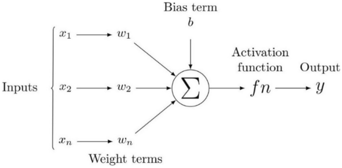
DNNs have been recognized as powerful tools that provide accurate predictions in classification and regression problems in several scientific fields. For example, DNNs have been applied in petroleum engineering to predict different reservoir rock properties from well-logging resistivity measurements, seismic data, and numerical or experimental measurements⁵⁶. Figure 6 presents an illustration defining the flow chart of neural networks. Here, all inputs are multiplied with their corresponding weights representing the strength of neurons and are controlled by a cost function. A weighted sum then adds together the multiplied values. The weighted sum is then applied to an activation function that delivers the network’s output. Considering a DNN with multiple output targets, the corresponding cost function based on mean square training errors is given as:

where \(\overset{\lower0.5em\hbox{$\smash{\scriptscriptstyle\frown}$}}{y}_{id}\) are the target values, and \(y_{id}\) are the network outputs associated with the network output \(k\) and training example \(d\). The gradient descent rule is used to find hypothesis values to the weights that will minimize \(J(\theta )\). Table 4 shows the backpropagation algorithm used to find these weights. The weight-update loop in backpropagation may be iterated thousands of times in a typical application. A variety of termination conditions can be used to halt the procedure.

The study also adopts DNNs as a regression approach to map the extracted features to absolute permeability and porosity. We train optimum DNN models (M₁–M₅) of a different number of hidden layers and the number of perceptrons in each layer to affect the model performance score. During the training of each model, we investigated and adopted the optimum hyperparameters of batch size, number of epochs, and a suitable optimizer for each model through a constrained randomized search (RSO) approach.

The ensemble stacking approach is designed to stack multiple predictions from three (3) linear and two (2) nonlinear machine learning-based models into a meta-leaner linear model (SMR-ML). The method is also designed to stack various predictions from multiple DNN networks of various levels of model complexity (the number of hidden layers and perceptrons per layer (Table 5). Individual predictions (\({P}_{1}-{P}_{5}\)) from the five DNN model (\({M}_{1}-{M}_{5}\)) architectures are stacked together into a meta-leaner linear model (SMR-NN). Each model is trained and saved independently on an optimum hyperparameter space in both stacking cases. To demonstrate the capabilities of the proposed approach, we select the multiple linear regression model (SMR) as the meta-learning model⁵⁷.

Hyperparameter tuning

Hyperparameters, such as the size of the network, the learning rate, the number of layers, and the type of activation function, control the learning process of a machine learning model. By adjusting these parameters, the model’s performance can be improved. Hyperparameter tuning, the process of identifying the best training hyperparameters of a single model, is tedious and usually based on trial and error. However, it is possible to recommend searching the hyperparameter space for the best hyperparameters that can deliver the best model score. Two generic tuning methods widely used include the exhaustive grid search (EGS) and the randomized parameter optimization (RSO). The EGS is a compelling approach but computationally expensive^58,59. In this study, we adopt the randomized parameter optimization method, which implements a randomized parameter search over selected model hyperparameters. Compared to the EGS, the addition of none influencing parameters into the pool of RSO-selected parameters does not affect the efficiency of the approach. Note that the selected best hyperparameters are entirely based on the dataset used and may change for other datasets.

Metrics and hyperparameters

This study adopts the mean squared error (MSE) as a loss function. MSE is widely used in ML-based regression models. The MSE gives the mean value of the square differences between the target set points and the regression line, expressed in Eq. (4).

Additionally, we adopt the mean absolute error (MAE) function (Eq. 5), a metric related to the mean of the absolute values of each prediction error on the test data. P is the property operator, which is a function of the inputs and the weights of the predictor network. This may also be identified as an activation function. Θ denotes the model weights, l_i represents the actual labels, and N represents the dataset size.

Typically, when conducting regression analysis with multiple inputs, it is advisable to rescale the input dataset to account for variations in their influence on the dependent variable⁶⁰. We tested various scaling techniques, including min–max scaling, absolute maximum scaling, and standardization. Based on our evaluation, standardization, which transforms the data to a normal distribution, yields the best results. Hence, we applied standardization (Eq. 6) to the dataset before training and evaluating the regression models discussed⁶¹. A dataset split of 80:20 in percentage is considered for the training and testing of the models. In Eq. (6), x represents the model inputs, µ denotes the mean, and σ is the standard deviation of the data.

The proposed models are trained and evaluated against test data using the coefficient of determination (R²) see Eq. (7). R² is a goodness-of-fit measure of the model predictions to the actual targets. It ranges between 0 and 1 or is expressed as a percentage. The higher the R², the more accurate the model is in predicting the targets, where \(y_{i} ,\overset{\lower0.5em\hbox{$\smash{\scriptscriptstyle\frown}$}}{y}_{i}\) and \(\overline{y}_{i}\) represent the targets, predictions, and mean values, respectively.

The proposed models are implemented using the Python platform. The RSO hyperparameter search is done using a single CPU node of a high-performance computer (HPC). Model training and testing were done using a NVidia GeForce Titan graphics card system with 12 Gigabyte memory, core i7 of 8th generation.