A light-weight, data-driven segmentation method for multi-state Brownian trajectories

Throughout this paper, we will consider the trajectory of a single Brownian particle which can adopt a number of discrete diffusive states i, each characterised by a self-diffusion coefficient D_i. The different states can, for example, model the binding and unbinding of a ligand to a receptor or the clustering between two protein molecules in a lipid bilayer, leading to a sudden change in diffusivity. The transition between states is described as a Poisson process with transition rates λ_ij, representing the probability per unit time of transitioning from state i to state j. For simplicity of presentation, our analysis will be restricted to the case of 2-state Brownian diffusion in 2 spatial dimensions, but the method can be generalised to higher-dimensional trajectories and/or higher numbers of states in a straightforward manner.

Model description

Synthetic, 2-state Brownian trajectories were generated by solving the discretised, overdamped Langevin equation using Euler’s method:

$${\boldsymbol{r}}({t}_{\alpha +1})={\boldsymbol{r}}({t}_{\alpha })+\sqrt{2{D}_{i}\delta t}{\boldsymbol{\omega }}({t}_{\alpha }),$$

(1)

where t_α = αδt is the discretised time, δt is the time step used to generate the trajectory (not to be confused with the microscope acquisition time, Δt, which we introduce below), and ω is a vector with the dimension of the system where each component is drawn from a normal distribution with zero mean and unit variance.

At each time step the particle changes its diffusion coefficient from D₁ (resp. D₂) to D₂ (resp. D₁) with a predefined transition rate λ₁₂ (resp. λ₂₁) with the transition probability³¹

$${p}_{12}=\frac{{\lambda }_{12}}{{\lambda }_{12}+{\lambda }_{21}}\left[1-\exp \left(-({\lambda }_{12}+{\lambda }_{21})\delta t\right)\right],$$

(2)

where p₁₁ = 1 − p₁₂ is the probability of remaining in state 1, and p₂₁ is obtained by interchanging the indices 1 and 2 in Eq. (2). The average lifetimes are furthermore given by ${\bar{\tau }}_{1}=1/{\lambda }_{12}$ and ${\bar{\tau }}_{2}=1/{\lambda }_{21}$.

To mimic the blur induced by the camera’s shutter count, following ref. ⁵⁴, we introduce the acquisition time Δt ≡ nδt, where the integer n is the number of discrete time steps over which the image is acquired. We assume constant illumination throughout the acquisition time Δt, meaning that all positions contribute equally to the average position measured over the time window. To mimic this process, we first generate a Brownian trajectory of length T by solving Eq. (1), which we then divide into T/n non-overlapping segments of length n, separated by Δt. The blurred trajectory is constructed by taking the arithmetic mean of the particle’s position within each segment. In addition, we mimic the errors introduced by limited spatial resolution and the subsequent tracking process by adding a Brownian noise ξ of zero mean and variance σ²³⁷. Taken together, the noisy trajectory $\bar{{\boldsymbol{r}}}$ is thus obtained as

$$\bar{{\boldsymbol{r}}}({\bar{t}}_{\alpha })=\frac{1}{n}\mathop{\sum }\limits_{m=0}^{n-1}{\boldsymbol{r}}({\bar{t}}_{\alpha }+m\delta t)+{\boldsymbol{\xi }}({\bar{t}}_{\alpha }),$$

(3)

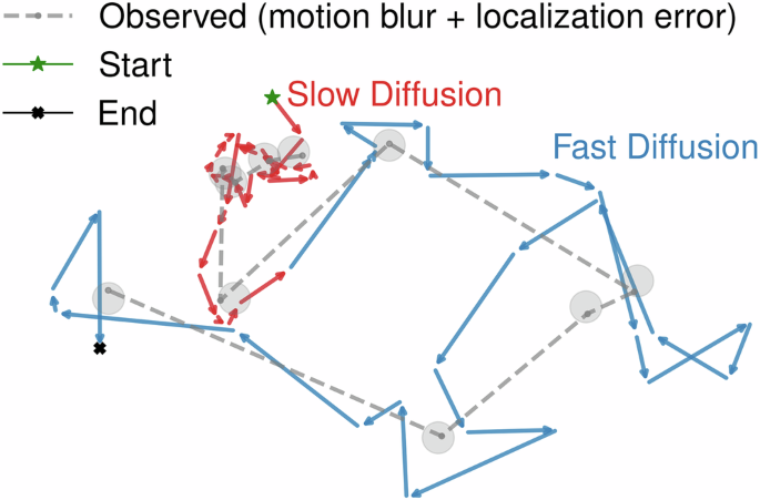
where ${\bar{t}}_{\alpha }\equiv \alpha \Delta t,\alpha =1,\ldots ,T/n$ now represents time measured in units of the camera acquisition time. This procedure introduces both temporal and spatial correlations into the trajectory, which must be considered when analysing the particle’s dynamics, such as determining the diffusion constant⁵⁴ or transition probabilities. An example of such a trajectory is presented in Fig. 1, illustrating the motion before and after the incorporation of motion blur and localisation error. In the following, we will use Δt as our basic time unit when presenting our data, unless stated otherwise.

Fig. 1: Example of a 2-state Brownian trajectory: The true trajectory is represented by colour-coded arrows, while the observed trajectory, shown as a dashed grey line with circular markers, is affected by motion blur (n = 5), where the path is averaged over non-overlapping time intervals.

Segmentation algorithm

The primary goal of the method is to infer the state of the particle at each time step based on its positional time series and the expected number of states. As schematically depicted in Fig. 2, we start by computing the displacement time series from the trajectory \(\bar{{\boldsymbol{r}}}
(4)

Fig. 2: Schematic of the different steps in the method: given a set of trajectories and an expected number of states, the overlap between the displacement distributions is minimised using an optimised Gaussian filter acting on the displacement time series.

Figure 3a shows an example of such a noisy time series, clearly showing a large spread across the two states. Since the displacements Δx and Δy in each dimension are normally distributed with mean μ_i = 0 and variance ${\sigma }_{i}^{2}\propto 2{D}_{i}$, the displacement probability distribution P_i(Δr) in state i of $\Delta r=\sqrt{\Delta {x}^{2}+\Delta {y}^{2}}$ is Rayleigh distributed, i.e.

$${P}_{i}(\Delta r)=\frac{\Delta r}{{\sigma }_{i}^{2}}\exp \left(-\frac{\Delta {r}^{2}}{2{\sigma }_{i}^{2}}\right),$$

(5)

yielding a 2-state displacement distribution given by

$$P(\Delta r)={\pi }_{1}{P}_{1}(\Delta r)+{\pi }_{2}{P}_{2}(\Delta r),$$

(6)

**Fig. 3: Segmentation of filtered displacement time series.**

with the weights π₁ = λ₂₁/(λ₁₂ + λ₂₁) and π₂ = λ₁₂/(λ₁₂ + λ₂₁) such that π₁ + π₂ = 1, as shown in Fig. 3b.

From Fig. 3a, b, we observe that, although large displacements are more frequent in the state with the higher diffusion coefficient, small displacements are frequent in both states, leading to considerable overlap between the two probability densities. Nevertheless, D₁ and D₂ can in principle be obtained by fitting the Rayleigh mixture model (RMM) in Eq. (6) to the measured distribution^16,35. However, the large overlap between the two probability densities makes a direct inference of the state at a given time point from the raw data challenging, and therefore, an RMM cannot be used directly to detect transitions or infer values of ${\bar{\tau }}_{i}$. To reduce this overlap and enable an explicit segmentation of the trajectory into a time series of the state of a given particle, we convolute the displacement time series Δr(t) with a discrete Gaussian filter β of width f to obtain the filtered displacement time series $\widehat{\Delta r}(t;f)$:

$$\widehat{\Delta r}({\bar{t}}_{\alpha };f)=\frac{{\sum }_{m=0}^{T}\Delta r({\bar{t}}_{m})\beta ({\bar{t}}_{\alpha }-{\bar{t}}_{m};f)}{{\sum }_{m=0}^{T}\beta ({\bar{t}}_{\alpha }-{\bar{t}}_{m};f)},$$

(7)

where $\beta (t;f)=\exp [-{t}^{2}/(2{f}^{2})]$. Here, we also tacitly assume that all state lifetimes ${\bar{\tau }}_{i}$ are longer than, or at least comparable to, the filter width f to avoid significant blurring of the state transitions.

This filtering procedure is a weighted, moving average, where the weights are given by a Gaussian distribution centred at each data point. In practice, this means that data points closer to the target point contribute more strongly to the filtered value, while points farther away contribute progressively less. For f ≪ Δt, β approaches a delta function, leading to a filtered displacement time series identical to the unfiltered one. Conversely, for f ≫ Δt, β yields an effectively constant displacement time series. For intermediate values, the temporal correlations introduced by the filtering process will reduce the standard deviation of P_i(Δr), leading to a decrease in the overlap between the individual probability distributions P₁ and P₂. This suggests that the overlap θ₁₂ between P₁ and P₂, which we use as an effective cost function, is minimised for some optimal value f* of the filter width. For values of f in the neighbourhood of f*, each point in the filtered displacement time series will therefore be influenced by only a small number of adjacent points in time, and the correlations introduced by the filtering are weak. In this case, the filtered sequence has enough independence that the central limit theorem applies, and $P(\widehat{\Delta r})$ can be accurately described by a sum of two Gaussian distributions ${\mathcal{N}}(\mu ,\sigma )$, according to

$$P(\widehat{\Delta r})\approx {\widehat{\pi }}_{1}{\mathcal{N}}(\widehat{\Delta r}| {\widehat{\mu }}_{1},{\widehat{\sigma }}_{1})+{\widehat{\pi }}_{2}{\mathcal{N}}(\widehat{\Delta r}| {\widehat{\mu }}_{2},{\widehat{\sigma }}_{2}),$$

(8)

with ${\widehat{\pi }}_{i}$ denoting the weights of the filtered displacement distribution for each state after the filtering process, and ${\widehat{\mu }}_{i}$, ${\widehat{\sigma }}_{i}$ the corresponding means and standard deviations, where ${\widehat{\pi }}_{i}\approx {\bar{\tau }}_{i}/({\bar{\tau }}_{1}+{\bar{\tau }}_{2})$ and we generally expect ${\widehat{\pi }}_{i}\approx {\pi }_{i}$ since the weights of the underlying two states are not altered by the filtering process. This decomposition allows us to use Gaussian mixture models (GMMs) for fitting the composite distribution. A GMM is a form of soft clustering that models data as a mixture of Gaussian distributions. Unlike hard clustering methods that assign each data point to a single cluster without accounting for any uncertainty in cluster membership, GMMs compute the probability p_i that a given data point (or displacement) belongs to each component (state) i in the mixture. The parameters of the model—the means, covariances, and weights—are estimated using the expectation-maximisation (EM) algorithm, which iteratively updates the probabilities of belonging to a given state and adjusts the model parameters to obtain an optimal fit^55,56; in our code, we use the GMM implementation provided by the GaussianMixture class in the scikit-learn library⁵⁷. GMMs are employed to fit the distribution $P(\widehat{\Delta r})$ and to provide a pointwise estimate of the likelihood p_i that a given displacement originates from a specific diffusive state i. This fitting procedure further enables an approximation of the overlap θ₁₂ between the two distributions, formally expressed as

$$\begin{array}{rcl}{\theta }_{12}(f) & \approx & \displaystyle{\int }_{-\infty }^{c}{\widehat{\pi }}_{1}{\mathcal{N}}(\widehat{\Delta r}(f)| {\widehat{\mu }}_{1},{\widehat{\sigma }}_{1})\,d\widehat{\Delta r}\\ & & +\displaystyle{\int }_{c}^{+\infty }{\widehat{\pi }}_{2}{\mathcal{N}}(\widehat{\Delta r}(f)| {\widehat{\mu }}_{2},{\widehat{\sigma }}_{2})\,d\widehat{\Delta r},\end{array}$$

(9)

where $c\in [{\widehat{\mu }}_{1},{\widehat{\mu }}_{2}]$ is the intersection point of the two weighted distributions, corresponding to the point where the probabilities of each of the two states are equal. For systems with multiple states, this generalises to the pairwise sum of the overlap, θ(f) = ∑_i>jθ_ij(f). Figure 3c shows the filtered version of the displacement distribution in Fig. 3b, which visually demonstrates the radically increased separability between the two states.

After finding f*, we obtain the time series representing the relative probability of each data point belonging to either of the two diffusive states, as illustrated in Fig. 3d. By assigning each filtered displacement to the state associated with the highest probability, we retrieve a segmented time series of the filtered displacements (Fig. 3e). Additionally, the pointwise probability values serve as quantitative indicators of the confidence associated with the state classification at each time point. In Fig. 3f, we show the resulting, inferred time series of the two diffusive states, together with the “ground truth” transition points used when generating the trajectory. In spite of the relatively large overlap between the unfiltered distributions (Fig. 3b), the reconstructed time series in Fig. 3f shows that all transitions are correctly detected within a small time window, indicating a successful segmentation of the trajectory. Here, we have also shown the time series of ${p}_{{\rm{mc}}}\equiv \min ({p}_{1},{p}_{2})$ inferred from Fig. 3d, which measures the a priori probability of misclassification at a given time point. The possibility to temporally monitor this measure provides a fast estimate of the quality of the data and the filtering. In the following section, we will quantify the accuracy of this segmentation and its dependence on the parameters of the problem.

Segmentation accuracy

In the following, we will demonstrate our method on 2-state Brownian trajectories generated as described in the previous section. Our main focus is on the discriminability between two states, quantified by the ratio of the two diffusion coefficients, $\widetilde{D}\equiv {D}_{{\rm{fast}}}/{D}_{{\rm{slow}}}$ and the shortest of the two lifetimes, $\widetilde{\tau }\equiv \min ({\bar{\tau }}_{1},{\bar{\tau }}_{2})$, measured in units of the shutter time Δt. The effect of the trajectory length, T, will also be examined, as well as the motion blur due to the limited shutter speed, as emulated by the averaging in Eq. (3), and the rescaled tracking error $\widetilde{\sigma }=\sigma /\sqrt{2{D}_{{\rm{slow}}}\Delta t}$.

We start in the absence of blurring and tracking error, corresponding to $\widetilde{\sigma }=0$ and n = 1 in Eq. (3), and investigate the accuracy of the segmentation for various values of $\widetilde{D}$ and $\widetilde{\tau }$. We define the accuracy as the proportion of time steps at which the inferred diffusive state matches the ground truth:

$$\,{\rm{Accuracy}}\,=\frac{1}{T-1}\mathop{\sum }\limits_{t=1}^{T-1}{\mathbb{1}}\left[{\widehat{s}}_{t}={s}_{t}\right],$$

(10)

where ${\widehat{s}}_{t}$ is the inferred diffusive state, s_t is the ground truth state at time t, and ${\mathbb{1}}[\cdot ]$ is the indicator function, which equals 1 if the prediction is correct and 0 otherwise. Parameter space was explored by generating N_t = 100 trajectories of length T = 1000 for each pair $(\widetilde{D},\widetilde{\tau })$. These parameters are important as $\widetilde{\tau }$ puts an upper bound on the range of possible filter size values before the filtering process starts to blur the two states, while $\widetilde{D}$ dictates the ideal filter size needed to minimise the overlap between the two states in the limit of very large $\widetilde{\tau }$.

Figure 4 a shows that our method gives a high precision segmentation (>90% accuracy) for a large range of ($\widetilde{D}$, $\widetilde{\tau }$), although it becomes inaccurate for a small separation between the diffusion coefficients ($\widetilde{D}\le 3$) or fast transition times compared to the camera resolution ($\widetilde{\tau }\le 20$). A trade-off between $\widetilde{D}$ and $\widetilde{\tau }$ is observed, as small values of $\widetilde{\tau }$ require a larger value of $\widetilde{D}$ and vice versa in order to effectively minimise the cost function and obtain an accurate segmentation. Figure 4b, c highlight the underlying optimisation algorithm behind the segmentation method, respectively showing the overlap θ₁₂ and the accuracy functions of the filter width f. First of all, we note that θ₁₂ is a convex function across the whole domain of interest, allowing for a well-posed optimisation problem. Secondly, there is a strong anticorrelation between the overlap and the segmentation accuracy for all parameter values shown, which supports our use of overlap as a cost function. Although the maximum in accuracy is not perfectly aligned with the minimum in θ₁₂, their colocalisation is strong enough to ensure a near-optimal performance in spite of the simplicity and fully automated nature of the optimisation method. The results further show that the optimal filter width is generally small, falling in the range 1 ≤ f ≤ 5, meaning that it is generally well-separated from the smallest transition time $\bar{\tau }$ apart from the smallest values explored in Fig. 4a.

**Fig. 4: Quantification of segmentation accuracy.**

In Fig. 4d, we furthermore demonstrate that the method is independent of the length of individual trajectories T. To verify this, we generate N_t trajectories of varying lengths T, keeping the total number of displacements N_t × T constant, fixed at 20,000 displacements. We observe that the accuracy of the segmentation method remains consistent regardless of trajectory length. While this might seem surprising, it is a direct consequence of the probabilistic nature of the segmentation method, which only relies on sampling a probability distribution of displacements between adjacent time points as in Fig. 3b, c, a process which does not require long individual time series. Therefore, the only strict requirement on the time series length for successful segmentation is that T ≫ f*. However, as we will see in the following section, a reliable estimate of the lifetimes ${\bar{\tau }}_{i}$ using the segmented trajectories imposes more conservative conditions on the trajectory lengths.

We now add the effect of localisation error and motion blur by generating N_t = 200 Brownian trajectories with T = 1000, $\widetilde{D}=4.0$ and $\widetilde{\tau }=20$, to which we apply different intensities of both spatial localisation error, as controlled by $\widetilde{\sigma }$, and motion blur, adjusted by changing n, the number of discretised steps over which the particle position in the original trajectory is averaged, when generating the trajectory according to Eq. (3). In Fig. 4e, we vary $\widetilde{\sigma }$ from 0, corresponding to no localisation error, to 2.1, corresponding to a case where the localisation error is significantly larger than the motion of the particle in its slowest state. The results show that the segmentation accuracy is essentially unaffected by the localisation error for $\widetilde{\sigma } < 1$. However, when $\widetilde{\sigma }\ge 1$, i.e., when the localisation error is of the order of the instantaneous displacement, the accuracy decays slowly, as expected. This is a consequence of the large noise introduced by the tracking error, which increases the overlap θ₁₂ and thus makes it harder to distinguish the two states from each other.

In Fig. 4f, we show the corresponding impact of the motion blur as quantified by the number of points n used to generate the rescaled trajectory in Eq. (3). Qualitatively, this yields a spurious correlation between adjacent displacements $\Delta r({\bar{t}}_{\alpha })$ and $\Delta r({\bar{t}}_{\alpha +1})$⁵⁴, which is generally challenging to handle using HMM-based methods³⁷. For our segmentation algorithm, the main effect is a slight blurring of the unfiltered probability distribution in Fig. 3b, which however does not lead to any measurable decline in the accuracy of segmentation, as shown in Fig. 4f. Unlike the localisation error σ, a direct translation of the parameter n to experimentally relevant ones is however not straightforward, as the underlying, discretised Brownian process used for the averaging is in itself not a faithful description of the real-world, continuous-time dynamics in the experimental system. Therefore, a continuous-time trajectory with motion blur corresponds to the limit n → ∞. For a full assessment of the impact of motion blur, a variation of the “blur factor”, R, which describes the impact of the shutter function on the trajectory, is therefore more appropriate, although also more technically complicated. The data generation in Eq. (3) corresponds to the simple case of giving equal weight to each position in the underlying trajectory, corresponding to a top-hat (or square-wave) shutter function that counts every photon during the acquisition time.⁵⁴

Extraction of dynamical properties

Once the trajectories have been segmented, the diffusion coefficient for each state can be directly determined from the corresponding trajectory segments. Since the segmented trajectories correspond to single-state ones, the dynamical analysis is significantly simplified, allowing for simple extraction of model parameters such as diffusion coefficients and state lifetimes. Assuming isotropic, Brownian diffusion, the displacements in each dimension can be utilised to compute the diffusion coefficient by averaging over both dimensions according to⁵⁴

$$\langle {\Delta }_{i}^{2}\rangle =2{D}_{i}\Delta t-2(2{D}_{i}R\Delta t-{\sigma }^{2}),$$

(11)

where $\langle {\Delta }_{i}^{2}\rangle$ is the mean-squared, unidimensional displacement averaged over the displacements corresponding to the i^th state and the blur factor R equals 1/6 if all frames are weighted equally during the acquisition process⁵⁴, as in Eq. (3).

To verify the accuracy of the parameter estimation, in Fig. 5a and b we extract the diffusion coefficient from 200 segmented trajectories with T = 5000, $\widetilde{D}=10.0$, and $\widetilde{\tau }=20$ using Eq. (11). Figure 5a shows that, even for low values of the localisation error, the faster of the two diffusion coefficients is systematically underestimated by ~ 10%. This is due to an asymmetry in the misclassification, whereby a larger part of the classification mistakes misclassifies displacements from the “slow” state as being “fast” than vice versa, resulting in a slight understimation of D_fast. On the other hand, the accuracy in determining D_i is suprisingly robust to the localisation error $\widetilde{\sigma }$: even when this is in the region $\widetilde{\sigma }\ge 1$ where classification errors start becoming significant (green curve in Fig. 4e), the impact on the predicted diffusion is negligible until $\widetilde{\sigma }\ge 1.5$, although its standard deviation (shaded regions in Fig. 5a) increases steeply with $\widetilde{\sigma }$, particularly for the slow state which gets the highest relative impact by the noise. This indicates that the additional classification errors introduced by localisation noise for moderate $\widetilde{\sigma }$ is symmetric in the sense that it leads to “fast” states being misclassified as “slow” ones as often as the opposite case, creating an effective cancellation of errors when calculating the diffusion coefficients. Figure 5b, which shows the effect of motion blur on the extraction of D_i, exhibits the same systematic underestimation of D_fast, although the accuracy is largely unaffected by the introduction of motion blur even as n → ∞. Importantly, this does not imply that motion blur does not affect the displacement time series, but only illustrates that this effect can be efficiently corrected for by the correction term in Eq. (11), since the calculation of D_i is done on the single-state trajectories after segmentation.

**Fig. 5: Extraction of dynamical variables after segmentation.**

Extracting the lifetimes of the two states is generally a much more demanding task, regardless of the segmentation method, as it intrinsically requires trajectories that are long enough to cover at least two transitions between the two states⁵⁰. Similar to previous methods⁵⁸, we estimate the average lifetime ${\bar{\tau }}_{i}$ by assuming a Poissonian behaviour and sampling the lifetime ${\tau }_{i}^{{\rm{m}}}$ of segmented trajectories, followed by fitting of the resulting histogram to an exponential distribution $P({\tau }_{i}^{({\rm{m}})})=\exp (-{\tau }_{i}^{({\rm{m}})}/{\bar{\tau }}_{i})/{\bar{\tau }}_{i}$, as shown in Fig. 5c. Compared to the determination of diffusion coefficients, this extraction is sensitive to errors in the segmentation process, since the misclassification of a displacement within a state introduces a “virtual transition”, leading to an underestimation of lifetimes, and primarily the lifetime ${\bar{\tau }}_{{\rm{fast}}}$ of the state with the faster diffusion. Nevertheless, Fig. 5d shows a relative error within ± 25% for τ ≥ 30, consistent with the trend observed in Fig. 4a, indicating that the method can provide reasonably accurate lifetime estimates if using sufficiently numerous and long trajectories. This also illustrates another advantage compared to fitting the unfiltered distribution to a Rayleigh mixture model, which does not enable the extraction of $\bar{\tau }$, but only of the ratio between the two lifetimes.

Experimental verification

The results in Figs. 3–5 all show examples of synthetic data, generated as discussed in the Model description section; in the following, we will illustrate the usability of our segmentation method also for experimental single-particle tracking data. To this end, we use a system consisting of Alexa Fluor 647-labelled, histidine-tagged SLAMF6 proteins (Catalogue #9299-NT, R&D Systems) anchored to a supported lipid bilayer, following the protocol described by Dam et al. ⁵⁹; a representative microscopy image of this system is shown in Fig. 6a. Visual inspection of the motion of the labelled proteins (Fig. 6b) indicates the presence of two different protein ensembles: one ensemble exhibiting free, 2-dimensional diffusion in the membrane and one with highly restricted mobility. In spite of this, the unfiltered displacement distribution in Fig. 6c shows a single, broad peak with an extended tail. The distribution is furthermore relatively poorly fitted by two Rayleigh distributions; in contrast, the filtered distribution (Fig. 6d) shows two well-separated, Gaussian peaks that are well-fitted by the GMM. The resulting diffusion coefficients, as calculated from Eq. (11), are D₁ = 0.057 μm² s⁻¹ and D₂ = 1.44 μm² s⁻¹, corresponding to $\widetilde{D}\approx 25$. This large ratio between the two particle mobilities, together with the fact that the two populations remain essentially constant over the course of the experiment, makes this a relatively “easy” system to segment, and further verification on experimental systems with dynamic binding-unbinding kinetics is clearly warranted. Nevertheless, the significant difference between the filtered and unfiltered distributions in Fig. 6 clearly illustrates the radical effect of our relatively simple segmentation algorithm when applied to experimental data.