CondensNet: enabling stable long-term climate simulations via hybrid deep learning models with adaptive physical constraints

CondensNet DL architecture and GCM model

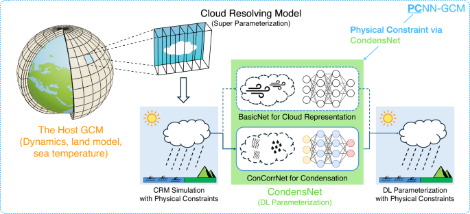
CondensNet (Fig. 5d) is a novel DL parametrization that learns and emulates the high-resolution CRM of SPCAM’s super parametrization⁸ (Fig. 5b), where the atmospheric dynamics is driven by the Community Atmosphere Model version 5.2 (CAM5.2)⁴¹ (Fig. 5e), running at a horizontal resolution of 1. 9° × 2. 5° with 30 vertical pressure levels, extending up to approximately 2 hPa, and employing a simulation timestep of 30 min. CAM5.2 is further coupled with the Community Land Model version 4.0 (CLM4.0)²⁸, using prescribed sea surface temperatures and sea ice concentrations according to the AMIP protocol.

Traditional GCMs like CAM use subgrid parametrization based on empirical models to represent cloud and convective processes (Fig. 5a), which can introduce significant uncertainties. GCMs that use super parametrizations, like SPCAM⁸, mitigate this issue by embedding a high-resolution cloud-resolving model (CRM) within each coarse grid cell (Fig. 5b). In our study, the two-dimensional CRM of SPCAM consists of 32 grid points in the zonal direction and shares 30 vertical levels with the host model dynamics driven by CAM5.2. The host GCM includes all model components except for the parametrizations, namely: the dynamical core, the land model (CLM4.0), and the sea surface temperatures. Consequently, SPCAM, CAM5.2, and the hybrid modeling framework share identical host GCM components and simulation data coupling workflows.

The host GCM provides input variables, including large-scale state variables such as water vapor Q, temperature T, surface pressure P_s, and top-of-atmosphere solar insolation Solin. In addition, large-scale forcing variables such as water vapor forcing dQ_l.s. and temperature forcing dT_l.s. are supplied to further enhance the model’s predictive capability. CondensNet, our DL parametrization, inherits these input variables and returns predictions of water vapor tendency dQ and dry-static-energy tendency ds at each vertical level, using an independent ResMLP model from ref. ²¹) to predict downwelling solar radiation fluxes to drive the coupled land surface model.

The complete list of inputs and outputs is provided in Table 2.

Our new DL parametrization, namely the CondensNet model, consists of two neural networks, that have different tasks, and are integrated together, as depicted in Fig. 5d. These are:

• BasicNet: tasked to predict basic tendencies of water vapor (dQ) and dry-static-energy (ds), capturing fundamental cloud physics. Here, we use the ResMLP model from ref. ²¹) as a basic model to explore the impact of ConCorrNet on stability in a more intuitive and controllable way.

• Condensation Correction Network (ConCorrNet): ConCorrNet is designed to predict physically-constrained corrections to BasicNet’s outputs. It is also an NN, operating as an independent, predictive module that is only activated adaptively in regions of unphysical atmospheric conditions (mainly oversaturation) to prevent model instabilities.

CondensNet predicts physically constrained tendencies of water vapor (dQ) and dry-static-energy (ds) that comply with the saturation adjustment mechanism, while the prediction of radiative fluxes remains untouched (i.e., not corrected), as depicted in Fig. 5d.

In particular, we identify oversaturated grid points by comparing the prognostic specific humidity (Q) with the saturation specific humidity (Q^*). A grid point is marked for subsequent adaptive physical constraint if it satisfies the condition Q > Q^*, which is equivalent to a relative humidity exceeding 100%. This process results in the creation of a humidity mask, (Mask_h):

where lon, lat, and lev represent the longitude, latitude, and vertical level indices of the grid points. The saturation specific humidity (Q^*) represents the maximum mass of water vapor that a unit mass of moist air can hold at a given temperature (T) and pressure (p). It is precisely defined and commonly approximated as:

where, p is the local atmospheric pressure, e^* is the saturation vapor pressure at temperature T (calculated using a formulation such as the Goff-Gratch equation⁴²), and ϵ = R_d/R_v ≈ 0.622 is the ratio of the specific gas constants for dry air (R_d) and water vapor (R_v).

We use Mask_h to mark regions where unphysical oversaturation is likely to occur; this marking directs ConCorrNet’s attention to these sensitive regions, but does not automatically enforce a correction. Instead, ConCorrNet consists of two neural networks that respectively predict the corrective tendencies dQ_fix and ds_fix. This adaptive methodology allows the model to learn the necessary physical corrections directly from the SPCAM labels for a given atmospheric state, enabling it to reproduce the complex physics of the reference simulation’s condensation processes.

In particular, the correction terms are then applied to the initial tendencies from BasicNet using the humidity mask Mask_h:

where ⊙ denotes element-wise multiplication. Through this mechanism, the physical constraints learned by ConCorrNet are integrated with the predictions from BasicNet. This ensures that the final outputs of the CondensNet model, the tendencies dQ_fixed and ds_fixed, are physically consistent. Following the methodology of Wang et al.²¹, the surface precipitation rate is then derived by vertically integrating CondensNet’s final prediction for the water vapor tendency, dQ_fixed. This process provides the necessary moisture source for the land and ocean components of the host GCM, thereby closing the water cycle.

To validate CondensNet and its ConCorrNet’s ability to enforce physical constraints and stabilize simulation, we used six ResMLP models from Wang et al.²¹ recorded as causing unstable simulations. With the weights of these unstable ResMLP models frozen to act as our BasicNet, we trained only the ConCorrNet module. This end-to-end training was guided by a unified loss function on the final, corrected tendencies (dQ_fixed, ds_fixed), ensuring that backpropagated gradients updated only ConCorrNet’s parameters. This experimental design isolates and demonstrates the corrective power of our module (i.e., six corrected cases in section “Long-term stability”). Further training specifications are provided in the subsection “Dataset and training details”.

Ablation studies presented in Supplementary Information Section C.2 further validate that correcting both dQ and ds is crucial for simulation stability.

Dataset and training details

CondensNet uses SPCAM simulation data for training. The specific inputs and outputs are listed in Table 2, including 30 vertical levels of specific humidity Q, temperature T, large-scale water vapor tendency dQ_l.s., large-scale temperature tendency dT_l.s., as well as single-level surface pressure P_s and single-level incoming solar radiation Solin. The spatial dimensions of the original SPCAM training data are detailed in Table 2. The original data were generated with a 30-min time step, the same as CAM5.2. Note that CondensNet is trained in a time-independent manner, with samples drawn directly from the SPCAM dataset.

The output variables are the corresponding tendencies of water vapor dQ and dry-static-energy ds at each vertical level (30 in total), as well as the four radiation fluxes (SOLS, SOLL, SOLSD, and SOLLD) in that reach to the surface.

Notably, in CondensNet, following the traditional column-based parametrization design in GCMs, each neural network instance processes a single atmospheric column independently. During training, column samples from different spatial locations are randomly shuffled, as the network only needs to learn the vertical physical processes within individual columns. When coupled to the host GCM, CondensNet instances operate independently on each column and physics time step. The exchange of mass, momentum, and energy between columns is mediated by the model dynamics, represented through the large-scale tendencies (input variables dQ_l.s. and dT_l.s.). This design maintains the intrinsic parallel efficiency of parametrizations while retaining the essential horizontal coupling provided by the dynamics.

The inputs consist of vertical profiles of atmospheric state variables (Q, T), large-scale tendencies (dQ_l.s., dT_l.s.), and surface conditions (P_s, Solin). The outputs include physical tendencies of water vapor (dQ) and dry-static-energy (ds) at each vertical level, along with surface radiation fluxes (summarized in Table 2).

The basic neural network, BasicNet, is a pre-trained Residual Multilayer Perceptron (ResMLP) that predicts basic tendencies of water vapor (dQ) and dry-static-energy (ds). It contains seven residual blocks (14 hidden layers in total) and two separate ResMLP neural networks—one for predicting dQ and one for ds. Each ResMLP module has 512 neurons for each hidden layer and uses ReLU activation functions.

The condensation correction network (ConCorrNet) is also a ResMLP designed to adjust the predictions of BasicNet to enforce physical constraints related to water vapor saturation. ConCorrNet architecture includes 6 residual blocks, each containing 2 fully connected layers with 512 neurons, resulting in a total depth of 12 hidden layers. We selected the sigmoid activation function based on its superior convergence performance observed in preliminary experiments.

In terms of training, we focus here on the definition and interpretation of the loss functions used to train CondensNet. BasicNet and ConCorrNet can be optimized either jointly or in a two-stage scheme in which BasicNet is pretrained and then frozen while training ConCorrNet. In this work, we adopt the latter for faster convergence; the mathematical objectives below apply to both training protocols.

We minimize a single supervised loss on the final, mask-corrected tendencies—dQ_fixed and ds_fixed—as defined in Eqs. (3) and (4), namely:

Here, N denotes the number of training samples (grid columns), and dQ_fixed and ds_fixed are the masked, physically corrected outputs of CondensNet. This formulation of the minimization problem allows the backpropagation of gradients to both BasicNet and ConCorrNet; the humidity mask then determines when and where ConCorrNet is active, and it needs to learn to correct BasicNet’s unphysical predictions.

To better understand the training strategy adopted, it is useful to express the minimization problem as the sum of two interpretable terms. First, the standard supervised loss for BasicNet

Second, the residual-regression objective for ConCorrNet, restricted to the oversaturated region identified by the binary mask Mask_h (with cardinality N_m):

Intuitively, if we interpret the humidity mask as a binary gate: when Mask_h = 1, ConCorrNet learns to correct the BasicNet predictions, while when Mask_h = 0 ConCorrNet is inactive. Accordingly, the implemented loss in Eq. (5) back-propagates gradients to both heads wherever Mask_h = 1, and to BasicNet everywhere. Details are provided in the Supplementary Information Section C.3.

The specific hyperparameters used during training for the results presented in this work are listed in Table 3, for both BasicNet and ConCorrNet.

The model was implemented using PyTorch and trained on multiple GPUs to accelerate computation. We used standard techniques such as data normalization and weight initialization to enhance training stability. Early stopping and model checkpointing were employed to prevent overfitting. The code is freely available at https://github.com/MathEXLab/PCNN-GCM.

Climatological processing

For variables with vertical distribution (temperature, wind speed, specific humidity), the zonal mean at each pressure level is given by

where N_λ is the number of longitudinal grid points, λ_i is the longitude at grid point i, ϕ is latitude, and p is pressure level. For surface or near-surface variables (precipitation, 10m wind speed), the horizontal mean is given by

where w(ϕ_j) is the latitudinal weight factor. The climatological means are then obtained by averaging these spatial means over the analysis period

where Y is the total number of years in the analysis period, X_m,y represents the monthly mean for month m in year y.

Error metrics

Once the means introduced in section “Climatological processing” are obtained, we use different error metrics to assess the performance of PCNN-GCM against NN-GCM and CAM5, using as a reference (i.e., ground truth) SPCAM. In particular, we use the pattern difference

where X_model and X_SPCAM represent the climatological means from a given model and SPCAM respectively, the weighted root mean squared error for variables with vertical distribution

where X₁ and X₂ represent the climatological means from two different models (for surface variables, the same formula applies without the pressure level dependency), and the coefficient of determination

where N is the total number of samples, \({X}_{i}^{{\text{model}}}\) and \({X}_{i}^{{\text{SPCAM}}}\) are the values at sample point i for a given model and SPCAM respectively, and \({\bar{X}}_{{\text{SPCAM}}}\) is the mean of SPCAM values over all samples.

In Eqs. (11–13), X_model corresponds to the model being evaluated (i.e., PCNN-GCM, NN-GCM, and CAM5), while X_SPCAM corresponds to the SPCAM reference (i.e., ground truth).