Regime-adaptive partial differential equations for interpretable multi-ethnic urban modeling

Multi-ethnic census dataset

Data sources and structure

We constructed a comprehensive multi-ethnic spatio-temporal dataset based on Statistics Canada census data spanning four census periods (2001, 2006, 2016, and 2021). The dataset captures population statistics disaggregated by ethnicity at the Dissemination Area (DA) level—the smallest standard geographic unit for census data dissemination, covering approximately 400–700 people per unit. For Toronto, this encompasses approximately 3700 DAs, providing high spatial resolution for analyzing urban dynamics.

The dataset includes detailed population counts for the five largest ethnic groups in Toronto: China, India, Philippines, Portugal, and Sri Lanka. While demographic features were normalized through standardization to ensure comparable scales across different variables, raw population counts were preserved to maintain the natural skewness of population distributions and allow the model to learn authentic patterns of concentration and dispersion. This structure allowed us to track three distinct temporal intervals (2001–2006, 2006–2016, and 2016–2021), reflecting different socioeconomic contexts and migration patterns.

Our analysis of the population distribution revealed significant variations across census periods. For example, the percentage of zero-population DAs (areas where specific ethnic groups are not present) decreased from 53.59 in 2001 to 24.39% in 2016, before increasing to 38.23% in 2021. This pattern reflects the complex dynamics of ethnic settlement and mobility, including colonization of new areas, concentration in existing enclaves, and exodus from certain neighborhoods. The population distribution exhibited high skewness (3.78–5.62) across all periods, indicating the presence of a small number of high-density ethnic clusters against a background of moderate-to-low density areas—a key challenge for conventional modeling approaches.

Feature Engineering

We extracted 298 socioeconomic and demographic features from the census data, organized into 12 categories:

1.

Demographics Population age structure, household composition, and family size
2.

Housing Dwelling types, ownership status, housing values, and maintenance needs
3.

Family Structure Marriage patterns, presence of children, household types
4.

Income Median household and individual income, income sources
5.

Employment Labor force participation, employment/unemployment rates
6.

Mobility & Migration Internal and external migration patterns, non-permanent residents
7.

Visible Minorities Population distribution by visible minority status
8.

Language Official language use, mother tongue, and multilingual capabilities
9.

Occupation Employment categories across economic sectors
10.

Religion Religious affiliations and practices
11.

Industry Distribution across industry sectors
12.

Place of Birth Country of origin information

To ensure temporal consistency, we selected features common across all census periods (2001–2021), which created a more stringent modeling challenge as recent census years (2016, 2021) contained additional variables that were excluded from the analysis. All features were standardized using z-score normalization to facilitate model training.

$${P}_{ij}= \left\{\begin{array}{c}1 \\ 0 \end{array}\genfrac{}{}{0pt}{}{\text{if DAs }i\text{ and }j\text{ share a boundary }\text{exp}(-|{x}_{i}-{x}_{j}{|}^{2}/{\sigma }_{p}^{2}) \text{if }|{x}_{i}-{x}_{j}|\le {d}_{\text{prox}} \, 0}{otherwise}\right.$$

Spatial data integration

We constructed three specialized spatial matrices to capture the complex spatial relationships between dissemination areas, building on established approaches in spatial statistics and urban modeling^22,28:

1.

Walking Distance Matrix Generated from Toronto’s street network using shortest-path algorithms to represent pedestrian connectivity between DAs. For each pair of DAs $(i,j)$, the matrix value was calculated as: ${W}_{ij}=\left\{\begin{array}{c}\text{exp}\left(-\frac{{d}_{ij}^{2}}{{\sigma }_{w}^{2}}\right) \text{if }{d}_{ij}\le {d}_{\text{max}} \\ 0 otherwise\end{array}\right.$ where ${d}_{ij}$ represents the shortest-path walking distance between the centroids of DAs, ${\sigma }_{w}$ is the distance decay parameter (1.5 km), and ${d}_{\text{max}}$ is the maximum connection distance (5 km).
2.

Transit Connectivity Matrix Incorporated public transportation routes from Open Data Toronto, representing the ease of movement between DAs via public transit: ${T}_{ij}= \left\{\begin{array}{c}\begin{array}{ccc}\text{exp}(-{t}_{ij}/{\sigma }_{t})& \text{if DAs }i\text{ and }j\text{ are connected by transit }& \end{array}\\ 0 otherwise\end{array}\right.$ where ${t}_{ij}$ is the travel time (in minutes) between DAs, and ${\sigma }_{t}$ is a time decay parameter (30 min).

Proximity Matrix: Captured geographic contiguity and straight-line distance:

${P}_{ij}= \left\{\begin{array}{c}1 \\ 0 \end{array}\genfrac{}{}{0pt}{}{\text{if DAs }i\text{ and }j\text{ share a boundary }\text{exp}(-|{x}_{i}-{x}_{j}{|}^{2}/{\sigma }_{p}^{2}) \text{if }|{x}_{i}-{x}_{j}|\le {d}_{\text{prox}} \, 0}{otherwise}\right.$ where ${x}_{i}$ and ${x}_{j}$ are the centroid coordinates, ${\sigma }_{p}$ is the distance decay parameter (0.8 km), and ${d}_{\text{prox}}$ is the maximum proximity connection distance (3 km).

Each matrix was constructed at 3742 × 3742 dimensions (covering all Toronto DAs), allowing comprehensive encoding of the urban spatial structure. These matrices enabled our model to incorporate physical barriers, transportation networks, and neighborhood adjacency—elements crucial for accurate population dynamics modeling but absent from traditional approaches.

Population change characterization

We conducted detailed analysis of population change patterns to inform our regime-specific modeling approach. For each temporal transition (2001 → 2006, 2006 → 2016, 2016 → 2021), we quantified:

1.

Zero-to-Non-Zero Transitions Representing colonization events where an ethnic group establishes presence in a previously uninhabited area. These transitions occurred in 44–68% of DAs across different periods.
2.

Non-Zero-to-Zero Transitions Representing complete exodus events where an ethnic group disappears from an area. These transitions ranged from 19 to 36% of DAs.
3.

Extreme Increases Population growth exceeding 100%, indicating rapid demographic shifts. These occurred in 7–14% of DAs.
4.

Extreme Decreases Population reduction exceeding 50%, indicating significant exodus. These occurred in 33–39% of DAs.

This analysis revealed substantial heterogeneity in population dynamics, reinforcing the need for regime-specific modeling approaches. For example, the 2006 → 2016 period showed the highest rate of zero-to-non-zero transitions (68.07% in training data), while the 2016 → 2021 period exhibited more balanced patterns between colonization and exodus dynamics.

Multi-ethnic spatial mixture of experts framework

Model architecture overview

The MESMoE model integrates physics-informed modeling with specialized expert systems to predict multi-ethnic population dynamics. The core innovation lies in the combination of a fundamental physics-based partial differential equation (PDE) framework with regime-specific expert models coordinated through a learnable routing mechanism inspired by the mixture of experts literature ^20,29 (see Supplementary Document Sect. 2 for detailed model foundation).

The model structure consists of:

1.

Feature embedding networks for environmental context
2.

Specialized expert modules for different population regimes
3.

A learnable router that determines expert utilization
4.

A physics-informed PDE solver for continuous dynamics
5.

An ethnicity interaction module capturing inter-group effects
6.

Area-specific parameter networks for spatial heterogeneity

Cultural-spatial resonance network

The foundation of our approach is the Cultural-Spatial Resonance Network (CSRN), which models population dynamics through a novel PDE formulation that extends traditional diffusion–reaction approaches ^21,24:

$$\frac{\partial {\phi }_{i}}{\partial t}={D}_{i}{\nabla }^{2}{\phi }_{i}+\nabla \cdot ({\lambda }_{i}{\mathbf{v}}_{i}\nabla {\phi }_{i})+(-{\alpha }_{i}(x,t)\cdot ({\phi }_{i}-{\overline{\phi }}_{i})-{\beta }_{i}

${\phi }_{i}(x,t)$ represents the population density

${D}_{i}$ is the diffusion coefficient

${\lambda }_{i}$ is the amplification factor

${\mathbf{v}}_{i}$ is the velocity field

${\alpha }_{i}\left(x,t\right)$ controls mean reversion

\({\beta }_{i}

${\gamma }_{i}$ modulates the advection stabilization

${K}_{i}$ is the gradient magnitude threshold

Unlike traditional PDEs for population dynamics that use constant parameters across space ²⁴, we introduce spatial dependency for the mean reversion term:

$${\alpha }_{i}\left(x,t\right)={\alpha }_{0,i}\cdot \text{exp}\left(-\frac{\| \nabla {\phi }_{i}{\| }^{2}}{{\sigma }_{i}^{2}}\right)$$

This formulation allows adaptive mean reversion based on local population gradients—a critical feature for capturing boundary dynamics between ethnic enclaves.

Mixture of experts framework

The complete model employs a mixture of experts architecture with four specialized expert models ^29,30:

$$\widehat{{\phi }_{i}}\left(t+\Delta t\right)=\sum_{e=1}^{4}{w}_{i,e}\cdot {E}_{e}\left({\phi }_{i}\left(t\right),\mathbf{f}\right)+{w}_{i,{\text{main}}}\cdot M\left({\phi }_{i}\left(t\right),\mathbf{f}\right)$$

where:

$\widehat{{\phi }_{i}}\left(t+\Delta t\right)$ is the predicted population for ethnicity $i$
${w}_{i,e}$ is the weight assigned to expert ee e for ethnicity $i$
${E}_{e}$ represents the expert models: colonization, jump process, decline, and PDE-based
$\mathbf{f}$ represents input features
$M$ is the main neural network
${w}_{i,{\text{main}}}$ is the weight for the main model

Expert weights are determined by a learnable router that maps feature and population states to expert assignment probabilities:

$${\mathbf{w}}_{i}={\text{Router}}\left({\phi }_{i}\left(t\right),\mathbf{f}\right)$$

The router incorporates domain knowledge through population threshold inductive biases:

$${\mathbf{h}}_{\text{hint}}=[{1}_{{\phi }_{i}\le {\theta }_{\text{col}}},{1}_{{\phi }_{i}>{\theta }_{\text{jump}}},{1}_{{\theta }_{\text{col}}<{\phi }_{i}\le {\theta }_{\text{decline}}},{1}_{{\theta }_{\text{col}}<{\phi }_{i}\le 2{\theta }_{\text{jump}}}]$$

where $1$ is the indicator function. The final expert weights blend learned probabilities with rule-based hints:

$${\mathbf{w}}_{\text{final}}=(1-\lambda )\cdot \mathbf{w}+\lambda \cdot {\mathbf{h}}_{\text{hint}}$$

where $\lambda$ is a blending parameter.

Specialized expert models

Multi-ethnic colonization expert

This expert handles zero-to-nonzero population transitions, modeling the initial establishment of an ethnic group in a previously uninhabited area based on concepts from colonization and diffusion of innovations theory^26,31. The colonization model predicts population establishment through a multi-stage hierarchical process:

$$p\left({\text{size}}|\mathbf{f}\right)={\text{Softmax}}\left({g}_{\text{size}}\left(\mathbf{f}\right)\right)$$

where $p\left({\text{size}}|\mathbf{f}\right)$ is the probability distribution over colonization sizes conditioned on features $\mathbf{f}$.

The predicted colonization value is:

$${\phi }_{i}^{\text{col}}=\sum_{s\in \left\{{\text{small}},{\text{medium}},{\text{large}},\text{very large}\right\}}p(s|\mathbf{f})\cdot ({h}_{s}(\mathbf{f})\cdot {\text{scale}}_{s}+{\text{bias}}_{s})$$

where ${h}_{s}$ are size-specific neural networks, and ${\text{scale}}_{s}$ and ${\text{bias}}_{s}$ are learned parameters.

Multi-ethnic jump process expert

This expert models discontinuous jumps in population values that cannot be captured by continuous diffusion processes, extending stochastic jump process theory³² to the spatial-ethnic domain. The jump process combines regular and extreme jump components:

$${\phi }_{i}^{\text{jump}}={\phi }_{i}

Parameter-adaptive scaling The solver dynamically adjusts integration scales based on population magnitude and regime type. For log-space populations (colonization regime), diffusion coefficients are constrained to $D\in [\text{0.01,0.5}]$ and time steps reduced by 90% ($\Delta {t}_{\text{eff}}=0.1\Delta t$) to prevent exponential instabilities. For linear-space populations, adaptive scale factors ${\alpha }_{\text{scale}}=\text{min}(\text{3.0,100}/(\text{max}(\mid \phi \mid )+\epsilon ))$ normalize PDE terms across population ranges spanning 4 orders of magnitude.

Gradient and Laplacian regularization Spatial derivatives incorporate stabilizing perturbations: $\nabla \phi \leftarrow \nabla \phi +\mathcal{N}(0,{0.01}^{2})$ and ${\nabla }^{2}\phi \leftarrow {\nabla }^{2}\phi +0.05\cdot {\text{sign}}(\phi )$. Gradient magnitudes are clamped to $\parallel \nabla \phi {\parallel }^{2}\in [\text{0.05,5.0}]$(log-space) or $[\text{0.05,100}]$(linear-space), preventing runaway growth in steep population transitions characteristic of jump processes.

RK4 integration with fallback Fourth-order Runge–Kutta integration employs clamped intermediate stages: ${k}_{i}\in [-\text{1.0,1.0}]$ for log-space and $[-\text{10.0,10.0}]$ for linear-space. A forced minimum update $\Delta {\phi }_{\text{min}}=0.01\cdot {\text{sign}}(\phi +0.001)$ ensures non-zero gradient flow during training even in near-equilibrium states. If RK4 fails (e.g., NaN propagation), the solver automatically falls back to forward Euler with aggressive clamping: ${\phi }^{n+1}={\text{clamp}}({\phi }^{n}+\Delta t\cdot {k}_{1},[-\text{20,20}])$ for log-space.

**CUDA kernel safeguards** At the lowest computational level, custom CUDA kernels enforce adaptive gradient clipping (max gradient scales with population: $\mid {\partial }_{x}{\mid }_{\text{max}}=\text{max}(\text{10,0.5}\cdot \mid \phi \mid )$), finite-value verification (NaN/Inf replaced with zeros), and minimum perturbations (${\epsilon }_{\text{min}}=\text{max}(\text{0.001,0.01}\mid \phi \mid )$) to maintain differentiability throughout backpropagation.

MoE-specific stabilization Because the PDE expert operates alongside discrete experts (colonization, jump, decline) with differing output scales, we enforce regime-appropriate bounds: colonization outputs $\in [\text{10,2000}]$, jump outputs $\le 3{\phi }_{t}+100$, decline outputs $\le {\phi }_{t}+50$, and PDE outputs $\le 5{\phi }_{t}+100$. Expert weight smoothing (${w}_{t}=0.2{w}_{t-1}+0.8{w}_{t}$) prevents abrupt transitions that could destabilize the PDE solver when regime assignments change.

Stability validation Conservation checks after each forward pass verify mass conservation error ${\epsilon }_{\text{mass}}=\mid {\sum }_{i}{\phi }_{i}^{n+1}-{\sum }_{i}{\phi }_{i}^{n}\mid /{\sum }_{i}{\phi }_{i}^{n}<{10}^{-4}$ and energy conservation ${\epsilon }_{\text{energy}}=\mid {\sum }_{i}({\phi }_{i}^{n+1}{)}^{2}-{\sum }_{i}({\phi }_{i}^{n}{)}^{2}\mid /{\sum }_{i}({\phi }_{i}^{n}{)}^{2}<{10}^{-3}$. Across 3,700 DA-level predictions spanning 20 years, the PDE expert achieved mean ${\epsilon }_{\text{mass}}=2.3\times {10}^{-5}$ and ${\epsilon }_{\text{energy}}=4.7\times {10}^{-4}$, confirming numerical stability throughout training and inference.

Area-specific parameter learning

A key innovation in our approach is the learning of area-specific parameters through specialized neural networks, extending spatially varying coefficient models²² with deep learning:

$${\theta }_{i}^{(a)}={g}_{\theta }({\mathbf{f}}^{(a)})$$

where ${\theta }_{i}^{(a)}$ represents a parameter (e.g., diffusion coefficient) for ethnicity $i$ in area $a$, ${\mathbf{f}}^{(a)}$ are the features of area $a$, and ${g}_{\theta }$ is a neural network.

For the PDE solver, all key parameters are area-specific:

$${D}_{i}^{\left(a\right)}={g}_{D}({\mathbf{f}}^{\left(a\right)}{)}_{i}$$

$${\lambda }_{i}^{\left(a\right)}={g}_{\lambda }({\mathbf{f}}^{\left(a\right)}{)}_{i}$$

$${\mathbf{v}}_{i}^{\left(a\right)}={g}_{v}({\mathbf{f}}^{\left(a\right)}{)}_{i}$$

$${\alpha }_{i}^{\left(a\right)}={g}_{\alpha }({\mathbf{f}}^{\left(a\right)}{)}_{i}$$

$${\beta }_{i}^{\left(a\right)}={g}_{\beta }({\mathbf{f}}^{\left(a\right)}{)}_{i}$$

$${\gamma }_{i}^{\left(a\right)}={g}_{\gamma }({\mathbf{f}}^{\left(a\right)}{)}_{i}$$

where each $g$ function is a neural network that maps area features to ethnicity-specific parameters.

Ethnicity interactions

Our model captures inter-ethnic influences through a learned interaction module inspired by social interaction models³⁷:

$${\mathbf{I}}_{i,j}=\sigma \left({g}_{\text{interaction}}\left({\varvec{\phi}}\right)\right)$$

where ${\mathbf{I}}_{i,j}$ represents the influence of ethnicity $j$ on ethnicity $i$. The interaction effect is computed as:

$${\mathbf{e}}_{i}=\sum_{j\ne i}{\mathbf{I}}_{i,j}\cdot ({\hat{\phi }}_{j}(t+\Delta t)-{\phi }_{j}

Pre-training Phase Initially, only the main neural network component was trained while keeping expert modules fixed.

Expert Training Phase The colonization expert was introduced first, followed by the PDE expert, and finally the jump and decline experts.

Router Training Phase Once all experts were trained, the router was fine-tuned to optimize expert assignment.

Full Model Fine-tuning All components were jointly optimized with a reduced learning rate.

Hyperparameter search framework and result is provided in Supplementary Document Sect. 5.

Loss function design

The model employed a multi-component loss function addressing the heterogeneous nature of population dynamics:

$${\mathcal{L}}_{\text{total}}={\mathcal{L}}_{\text{prediction}}+{\lambda }_{\text{aux}}{\mathcal{L}}_{\text{auxiliary}}+{\lambda }_{\text{reg}}{\mathcal{L}}_{\text{regularization}}+{\lambda }_{\text{phys}}{\mathcal{L}}_{\text{physics}}+{\lambda }_{\text{cons}}{\mathcal{L}}_{\text{conservation}}$$

The core prediction loss used a regime-adaptive weighting scheme:

$${\mathcal{L}}_{\text{prediction}}=\frac{1}{B\cdot E}\sum_{b=1}^{B}\sum_{e=1}^{E}{w}_{b,e}\cdot {w}_{e}\cdot ({\hat{\phi }}_{b,e}-{\phi }_{b,e}{)}^{2}$$

where ${w}_{b,e}$ are case-specific weights determined by population regime:

$$\begin{gathered} w_{{b,e}} = \{ w_{{{\text{col}}}} {\text{if }}\phi _{{b,e}}^{{{\text{init}}}} \le \theta _{{{\text{col}}}} {\text{(colonization case) }}w_{{{\text{jump}}}} {\text{if }}\phi _{{b,e}}^{{{\text{change}}}} \theta _{{{\text{jump}}}} {\text{(jump case) }}w_{{{\text{decline}}}} \hfill \\ {\text{if }}\phi _{{b,e}}^{{{\text{init}}}} \le \theta _{{{\text{decline}}}} {\text{ and }}\phi _{{b,e}}^{{{\text{change}}}} \le 0{\text{(decline case) }}w_{{{\text{pde}}}} \hfill \\ {\text{if}}\;{\text{case}}\;{\text{meets}}\;{\text{PDE}}\;{\text{criteria(PDE case) }}1.0\;{\text{otherwise (regular case)}} \hfill \\ \end{gathered}$$

The optimal weight values determined through ablation studies are ${w}_{\text{col}}=5.0$, ${w}_{\text{jump}}=3.0$, ${w}_{\text{decline}}\boldsymbol{}=4.0$, and ${w}_{\text{pde}}\boldsymbol{}=2.0$.

For jump cases, we applied an additional log-space transformation to better handle large magnitude changes:

$${\mathcal{L}}_{\text{jump}}=(log({\hat{\phi }}_{b,e}+1)-log({\phi }_{b,e}+1){)}^{2}\cdot 100.0$$

The auxiliary loss guides the expert router to correctly classify population dynamics:

$${\mathcal{L}}_{\text{auxiliary}}=-\frac{1}{B\cdot E}\sum_{b=1}^{B}\sum_{e=1}^{E}\sum_{c=1}^{C}{y}_{b,e,c}\text{log}({p}_{b,e,c})$$

The physics-informed loss enforces consistency with the underlying PDE:

$${\mathcal{L}}_{\text{physics}}=\frac{1}{B\cdot E}\sum_{b=1}^{B}\sum_{e=1}^{E}{1}_{\text{isPDE}}(b,e)\cdot {\| \frac{\partial {\phi }_{b,e}}{\partial t}-F({\phi }_{b,e},\nabla {\phi }_{b,e},{\nabla }^{2}{\phi }_{b,e})\| }_{2}^{2}$$

Optimization strategy

We used Adam optimizer⁴⁰ with weight decay regularization and a learning rate schedule combining warm-up and cosine annealing⁴¹:

$${\eta }_{t}=\left\{\begin{array}{c}{\eta }_{\text{max}}\cdot \frac{t}{{T}_{\text{warmup}}} {\text{i}}{\text{f}} \, t\le {T}_{\text{warmup}} \\ {\eta }_{\text{min}}+\frac{1}{2}\left({\eta }_{\text{max}}-{\eta }_{\text{min}}\right)\left(1+\text{cos}\left(\pi \frac{t-{T}_{{\text{w}}{\text{armup}}}}{T-{T}_{\text{warmup}}}\right)\right){\text{o}}{\text{t}}{\text{h}}{\text{e}}{\text{r}}{\text{w}}{\text{i}}{\text{s}}{\text{e}}\end{array}\right.$$

where ${T}_{\text{warmup}}$ is the warm-up period length (typically 5 epochs), $T$ is the total number of epochs, ${\eta }_{\text{max}}$ is the maximum learning rate (0.0005), and ${\eta }_{\text{min}}$ is the minimum learning rate (0.00001).

To ensure training stability, we implemented adaptive gradient clipping with threshold:

$$\tau =max(0.1,min(5.0,\frac{\| \theta {\| }_{2}}{100}))\cdot {\tau }_{\text{base}}$$

with ${\tau }_{\text{base}}$$=5.0$ as the base clipping threshold.

Cross-temporal validation

To evaluate the model’s ability to predict across different temporal intervals, we employed a cross-temporal validation strategy:

1.

Within-Period Validation For each temporal period (2001–2006, 2006–2016, 2016–2021), we trained separate models using 80/20 train-test splits of dissemination areas from that specific period. This approach, which forms the basis for results in Table 1, ensures fair comparison across model architectures under consistent socioeconomic conditions by isolating model quality from temporal transfer effects.
2.

Cross-Period Validation We evaluated models trained on one period against test data from different periods to assess temporal generalization across nine distinct train-test combinations. Results reveal temporal resolution as the dominant factor affecting cross-period transfer. When PDE time steps match (5 → 5 year), models achieve strong bidirectional generalization: the 2016–2021 model maintains R² = 0.74 on 2001–2006 data (9% degradation), while the 2001–2006 model achieves R² = 0.70 on 2016–2021 data (14% degradation), demonstrating robust performance across 15–20 year temporal gaps with a modest 4% asymmetry favoring recent models. However, temporal resolution mismatches cause substantial degradation: 5 → 10 year transfers achieve R² = 0.25–0.43 (47–67% degradation), while 10 → 5 year transfers achieve R² = 0.45–0.54 (29–44% degradation). This sensitivity reveals a critical operational constraint: models must be trained on periods matching intended prediction horizons for reliable performance (see Supplementary Materials Sect. 3.2.6 and Table S1 for complete validation matrix).
3.

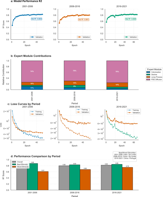
Multi-Period Training We explored training on combined data from multiple periods (2001–2006 + 2006–2016) to assess benefits of incorporating diverse temporal dynamics. The multi-period model achieved R² = 0.68 on 2016–2021 test data, representing intermediate performance between temporally-matched single-period models (R² = 0.74) and mismatched transfers (R² = 0.25–0.45). This demonstrates feasibility but reveals that temporal resolution matching provides clearer benefits than expanded training data, establishing period-specific training as the preferred approach for within-period prediction accuracy. The comprehensive validation results (Supplementary Table S1) demonstrate that MESMoE achieves excellent within-period performance (R² = 0.71–0.81) across three distinct socioeconomic eras while maintaining reasonable cross-period generalization when temporal resolution and feature availability are matched. Detailed analysis of cross-period performance patterns, architectural considerations, and practical application guidelines are provided in Supplementary Materials Sect. 3.2.6.

For each temporal period, we used an 80/20 train/test split, with the training data further divided into 90% training and 10% validation. Model performance was evaluated using multiple metrics, including Mean Squared Error (MSE), Mean Absolute Error (MAE), and coefficient of determination (R²), both overall and disaggregated by ethnicity and population dynamic regime. It is important to note that our validation approach assesses predictions at census intervals (5 or 10 years) due to ground truth data availability, rather than at intermediate time points. While the Cultural-Spatial Resonance Network’s continuous PDE formulation theoretically enables predictions at arbitrary time points through its Runge–Kutta integration, census data—the gold standard for population statistics—is only collected at 5-year intervals, providing ground truth observations exclusively at census years. The model predicts population distributions at the next census time point given the current census as input, but intermediate-year predictions (e.g., 2003, 2004) cannot be empirically validated against observed data. This validation constraint reflects: (1) the discrete nature of census data availability, which provides no ground truth for intermediate years, (2) the resulting inability to train or validate the model on sub-census-interval predictions, and (3) the alignment with urban planning practice, where major policy decisions typically operate on 5–10 year planning horizons synchronized with census data releases. Future work incorporating auxiliary data sources (annual population estimates, building permits, administrative records) could enable intermediate-year validation, but current empirical validation necessarily focuses on census endpoints where observed data exists.

Interpretability analysis framework

We developed a comprehensive interpretability framework to analyze the learned model components:

1.

Feature Importance Analysis Computed based on the magnitude of weights in the first layer of each expert module⁴².
2.

Expert Contribution Analysis Quantifying the relative contribution of each expert to the final predictions.
3.

Ethnicity Interaction Analysis Measuring the strength and direction of inter-ethnic influences through interaction matrices.
4.

Spatial Parameter Visualization Creating high-resolution maps of physics-informed parameters across urban space.

The framework enables quantitative assessment of the socioeconomic drivers of population dynamics, the relative importance of different demographic mechanisms, and the spatial heterogeneity of population processes across urban neighborhoods.

Source link

Regime-adaptive partial differential equations for interpretable multi-ethnic urban modeling

Multi-ethnic census dataset

Data sources and structure

Feature Engineering

Spatial data integration

Population change characterization

Multi-ethnic spatial mixture of experts framework

Model architecture overview

Cultural-spatial resonance network

Mixture of experts framework

Specialized expert models

Multi-ethnic colonization expert

Multi-ethnic jump process expert

Area-specific parameter learning

Ethnicity interactions

Loss function design

Optimization strategy

Cross-temporal validation

Interpretability analysis framework

RECENT POSTS

YouTube AI similarity detection tool helps creators remove deepfake videos

3 reasons why Amazon is a top AI investment

I left Google after 18 years. I felt pressure to implement AI quickly.

Multi-ethnic census dataset

Data sources and structure

Feature Engineering

Spatial data integration

Population change characterization

Multi-ethnic spatial mixture of experts framework

Model architecture overview

Cultural-spatial resonance network

Mixture of experts framework

Specialized expert models

Multi-ethnic colonization expert

Multi-ethnic jump process expert

Area-specific parameter learning

Ethnicity interactions

Loss function design

Optimization strategy

Cross-temporal validation

Interpretability analysis framework

Related Posts