
This section discusses the clustering analysis and validation of defect clusters based on the feature model proposed above and further designs a modular defect cluster configuration recognition algorithm. First, a comparison is made between the t-SNE and UMAP dimensionality reduction methods regarding their strengths and weaknesses in preserving global structural information and handling defect data. Then, a comparison is made between the feature models based on adjacent points and those based on centroids in terms of clustering effectiveness. In addition, by incorporating the dual-pointer lattice filling method, the identification of complex defect structures is further realized, improving the accuracy of analyzing defect morphology and distribution characteristics.
Defect clustering analysis and verification based on the feature model
Comparison of dimensionality reduction results
The dimensionality reduction results are shown in Fig. 10a,b, where the horizontal and vertical axes are abstract and do not represent physical coordinates. Each point denotes a defect cluster, and the colors distinguish between vacancy clusters (yellow) and interstitial clusters (blue), defined based on the relative number of vacancy and interstitial atoms. Notably, even though the features used for dimensionality reduction were not explicitly designed to separate these two categories, the projected distributions show a clear separation between the two. This indicates that the structural characteristics captured in the high-dimensional space intrinsically differ between vacancy and interstitial clusters, and that the feature vectors encode meaningful physical or geometrical differences.

Dimensionality reduction results with the t-SNE and the UMAP algorithm.
To investigate the separability and structural patterns of defect clusters, we employed two widely-used nonlinear dimensionality reduction methods: t-SNE and UMAP. These techniques are particularly suitable for high-dimensional, nonlinearly separable data, which is common in molecular dynamics simulations.
Although the visual results from both methods demonstrate clear separation, UMAP presents several technical advantages that justify its selection for further clustering. Specifically, UMAP tends to produce smoother and more consistent boundaries between clusters, as well as tighter intra-cluster distributions. It also preserves more of the global structure of the data, which is valuable for clustering algorithms such as HDBSCAN that rely on spatial continuity and density. In contrast, t-SNE often emphasizes local neighborhood structure at the expense of global layout, and its results can be more sensitive to initialization and perplexity settings. These advantages−together with its robustness and better preservation of both local and global topologies−make UMAP more suitable for our workflow, especially when coupled with density-based clustering methods in subsequent analysis steps.
Validation of the clustering model
To verify that the optimized feature model proposed in Section *Feature Engineering and Feature Selection* is more conducive to clustering defect clusters, an experimental comparison was conducted between the centroid-based method and the adjacent-point-based method. HDBSCAN was uniformly used for clustering analysis, and the number of clusters labeled as “-1” and the silhouette coefficient values were calculated, as shown in Table 9. Clusters labeled “-1” are considered noise points. The dataset contains a total of 3,632 defect clusters. From the table, it can be seen that using centroid-based feature vectors for clustering resulted in 219 clusters being classified as noise, whereas the adjacent-point-based feature vector method reduced the noise, ensuring that more cluster structures were effectively classified and identified. Additionally, the silhouette coefficient, as an evaluation metric for clustering performance, was higher for the adjacent-point-based method than for the centroid-based method, indicating better clustering performance for the former. This further proves the applicability and robustness of the defect cluster structural feature representation method proposed in this paper.
Optimization of the component-based cluster identification algorithm
The structure of defect clusters has a significant impact on the migration rate, interaction, and annealing behavior of defect atoms during irradiation damage. Unsupervised cluster clustering can only classify clusters with simple morphologies and cannot identify more detailed internal configurations within clusters. For example, clustering alone cannot identify defect clusters composed of several complexly arranged and scattered self-interstitial atoms. Based on the clustering analysis in Section *Defect clustering analysis and verification based on the feature model*, more detailed identification of defect structures is needed to better explore the evolution patterns of defect structures and irradiation damage mechanisms, thereby enabling longer time-scale predictions of microstructural evolution. In metallic crystalline materials, various defect morphologies exhibit unique, well-defined structural shapes under stable conditions. Therefore, by defining the typical configurations of defect clusters, basic rules for the morphological characteristics can be established to recognize the internal configuration of defect clusters.
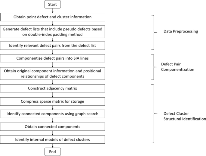
To achieve more accurate cluster recognition, this section further designs and implements a defect cluster configuration recognition method based on the findDefects set and the allClusters set, with the specific steps shown in Fig. 11. The method identifies the internal configuration of defect clusters through three steps: obtaining defect pairs, modularizing defect atoms, and identifying and finding connected components. Through the centralized construction of typical cluster configurations, automatic recognition is achieved.
Cascade defect cluster recognition and analysis process.
Defect cluster componentization
There are many smileyface_type defects and glasses_type pairs composed of defects and pseudo-defects in the cluster, with the corresponding defects represented by the glasses_type and smileyface_type in the allClusters set, as shown in Fig. 12a,b. Based on the specific positional relationship between smileyface_type defects or glasses_type pairs, they are defined as a single component called an SIA (Self-interstitial Atom) line, which consists of several smileyface_type defects or glasses_type pairs arranged collinearly. This allows the point defects to be associated according to their arrangement, facilitating the implementation of the subsequent defect configuration recognition algorithm.

Smileyface_type defects and glasses_type pairs.
(1) Defect Statistics Method Based on Wigner-Seitz (W-S) Cell Optimization To identify defect configurations, a different statistical method from the Frenkel defect pair method is required to group all defect atoms, including defect atoms and pseudo-defect atoms−such as extra interstitial-vacancy pairs. This is crucial for describing defect configurations. For example, in the glasses_type pairs shown in Fig. 12b, which is a type of interstitial-vacancy pair, it consists of three interstitial atoms and two vacancies. The net number of defect atoms in this type of defect pair is one, but the pseudo-interstitial and pseudo-vacancy included in the pseudo-defect structure configuration will help identify the configuration.
This statistical method associates each atomic coordinate with its nearest lattice point. If multiple atoms are related to a single lattice point, all related atom coordinates and the lattice point are added to the defect list, while marking the closest atom and lattice point as pseudo-defects. These pseudo-defects are not counted in the total number of defects or in the size of the defect cluster. The detailed steps for defect statistics are described below.
The W-S cell is a commonly used geometric construction for studying crystalline materials. The 2D construction method is shown in Fig. 13. First, a lattice point is selected, and lines are drawn connecting it to all its nearest neighbor lattice points. Perpendicular bisectors are then drawn for each line, and the resulting enclosed region is the W–S cell.

Schematic diagram of the two-dimensional structure of the W–S primitive cell.
The idea behind defect analysis using the W–S cell method is to calculate the distance between the current atom and each lattice point in the crystal, and then select the nearest lattice point as the occupied point. The current atom is compared with the previously occupied lattice points, and if it occupies the same point as a previous atom, the current atom is marked as a defect atom. After traversing all the atoms, if there are lattice points that are not occupied by any atom, those lattice points are marked as vacancies and are considered defect atoms as well. The schematic is shown in Fig. 14. Among them, the mark 1 represents a normal lattice atom, the mark 0 represents a vacancy, and the mark greater than 1 represents an interstitial atom.

Schematic diagram of defect analysis using the W–S primitive cell method.
One limitation of this method is that it requires comparing each atom with all previously occupied lattice points, resulting in a time complexity of \(O(N^2)\).
In this paper, we improve the W-S cell method by adding the labeling of pseudo-defects. When there is more than one atom in a cell, the lattice point is marked as a pseudo-vacancy, one atom is marked as a pseudo-interstitial, and the remaining atoms are marked as interstitials. The introduction of pseudo-defects allows for a more complete representation of the internal configuration of clusters, making it possible to identify Smileyface_type defects, glasses_type pairs, or more complex ring structures.
We further improve the algorithm based on the W-S cell method, which we call the dual-pointer lattice filling method. The main idea is to traverse both atoms and lattice points in an orderly manner. All atoms are sorted based on the coordinates of their occupied lattice points, in ascending order of z, y, and x coordinates. Dual pointers are set to traverse the atoms and lattice points simultaneously. If the current atom occupies the same lattice point as the current lattice point, both pointers move forward simultaneously. If the current atom’s occupied lattice point is ahead of the current lattice point, the lattice point pointer is advanced until they match, marking all intermediate lattice points as vacancies. If the current atom’s occupied lattice point is behind the current lattice point, the atom is marked as an interstitial, the atom occupying that lattice point is marked as a pseudo-interstitial, and that lattice point is marked as a pseudo-vacancy.
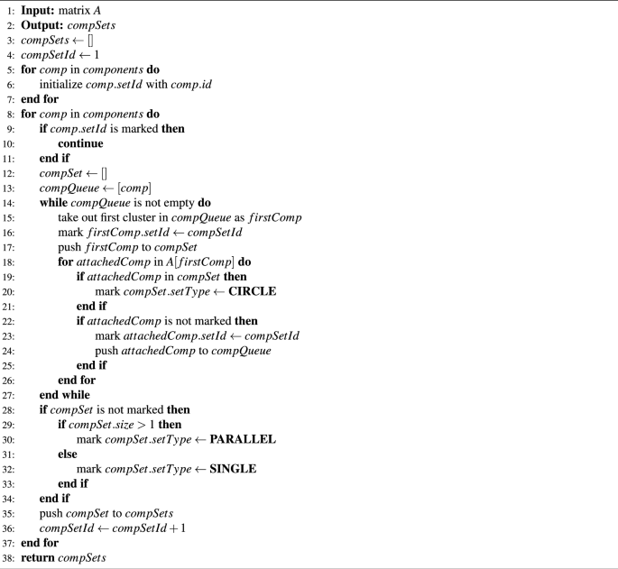
The pseudo-interstitial-vacancy pairs introduced by this method are not included in the count of defect atom pairs, but they play an important role in subsequent configuration recognition, helping to better represent the defect configuration and distribution characteristics. The time complexity of this method is \(O(N \log N)\), and it requires constant-level additional storage, making it well-suited for identifying defect cluster structures in large numbers of atoms. The pseudocode for this algorithm is shown in Algorithm 4.
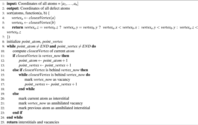
Double Pointer Lattice Filling Method
The steps of the pseudocode are explained in detail below:
Step 1: Sorting all atoms in the defective crystal, using the coordinates of their nearest lattice point as the sorting criterion. The nearest lattice point coordinates are calculated based on the distance between the atom and each lattice point within the cell. The atom’s cell coordinates, \(\vec {x}_{\text {cell}}\), are first calculated as equation 4:
$$\begin{aligned} \vec {x}_{\text {cell}} = \left\lfloor \frac{\vec {x}_{\text {atom}}}{\text {latticeConst}} \right\rfloor \end{aligned}$$
(4)
Next, the relative coordinates of the atom, \(\vec {x}_{\text {atom}\_\text {inside}} = [x_1, x_2, x_3]\), within the unit cell are calculated as equation 5:
$$\begin{aligned} \vec {x}_{\text {atom}\_\text {inside}} = \frac{\vec {x}_{\text {atom}} \bmod \text {latticeConst}}{\text {latticeConst}} \end{aligned}$$
(5)
A relative coordinate system can then be established within the unit cell, mapping the unit cell into a cube with an edge length of 1, with the atom located inside this cube. First, the distance between the atom’s coordinates \(\vec {x}_{\text {atom}\_\text {inside}}\) and the center lattice point coordinates \(\vec {x}_{\text {center}\_\text {inside}} = [0.5, 0.5, 0.5]\) is calculated as the reference value \(d_0\), as shown in equation 6:
$$\begin{aligned} d_0 = \left\| \vec {x}_{\text {atom}\_\text {inside}} – \vec {x}_{\text {center}\_\text {inside}} \right\| _2 \end{aligned}$$
(6)
Next, the distances between the atom and the lattice points at each vertex are calculated using the mirror method to directly select the nearest vertex lattice point. Since the atom is inside a cube, its distance to each vertex can be broken down into the sum of the squares of the perpendicular distances to the three planes containing the vertex. Starting from the origin [0,0,0], the perpendicular distance to each plane is considered separately. If the perpendicular distance exceeds latticeConst/2, the plane is switched to the mirror plane of the cube, and the target vertex is changed to the one at the intersection of the three planes. In this case, the coordinate value for the corresponding dimension is set to 1. This process ultimately yields the nearest distance \(d_{\min }\) and the closest lattice point vertex, as shown in equation 7:
$$\begin{aligned} d_{\min } = \sqrt{\left( \min \left\{ x_1, 1 – x_1\right\} \right) ^2 + \left( \min \left\{ x_2, 1 – x_2\right\} \right) ^2 + \left( \min \left\{ x_3, 1 – x_3\right\} \right) ^2} \end{aligned}$$
(7)
Based on the nearest vertex lattice point distance and the center lattice point distance, the atom’s nearest neighbor lattice point can be selected. Then, the z, y, and x coordinates of the nearest neighbor lattice point are used to sort the atoms in ascending order.
Step 2: A dual-pointer method is used to traverse both the atoms and the lattice points. The lattice point coordinates are incremented in z, y, and x order, scanning layer by layer. If the atom’s nearest neighbor lattice point is the current lattice point, it is determined that the atom occupies this lattice point, and both pointers are advanced simultaneously. If the atom’s nearest neighbor lattice point appears after the current lattice point, all lattice points between the current and target lattice points are marked as vacancies, and the lattice point pointer advances to the target lattice point. If the atom’s nearest neighbor lattice point appears before the current lattice point, it is determined that multiple atoms occupy the target lattice point. The current atom is marked as an interstitial, the target lattice point is marked as a pseudo-vacancy, and the atom occupying the target lattice point is marked as a pseudo-interstitial, with the atom pointer advancing by one position. After the traversal is complete, all vacancies and interstitials are identified.
The final defect list, codefects, is generated in array form. This array records the defect numbers, starting from 1. If the difference between consecutive numbers is 1, it indicates that the current lattice point is associated with only one defect atom. Otherwise, the number of defects at the current lattice point is greater than 1, generally 2 or 3, forming a smileyface_type or glasses_type clusters. When the number of defects corresponding to the same lattice point is 2, the two defect numbers are recorded and stored in the dictionary pairs. When the number of defects corresponding to the same lattice point is 3, the three defect numbers are recorded and stored in the dictionary glasses_type.
(2) Description of Defect Cluster Component Information Data
Defect component information is stored in the form of a JSON object, which includes the component ID, the defect point IDs that make up the component, subcomponent information under that component, directional information of the component, and individual scattered point defects.
Defects are organized into SIA (Self-Interstitial Atom) lines, and the relationships between lines are represented by a data structure called LinesData, as shown in Fig. 15. LinesData consists of lines and sub lines. A line may not always contain sub lines; only when two lines meet the merging rules does one line become the sub line of the other. The parameters in a line are as follows:

Organization of component information data.
-
id: The current SIA line’s ID.
-
eq: The coordinates of two points through which the SIA line passes.
-
points: An array of defect IDs.
-
angles: The angles between the current line and the x, y, and z planes, determining the direction of the line.
-
isVac: Determines whether two defects, when connected to a lattice point, form coincident lines.
-
vacErr: Represents the angle between the lines formed by two defects and the lattice point, and the distance between the lattice point and the lines connecting the two defects.
-
children: Contains the IDs of all sub lines within the line, as well as the distance from the main line to its sub lines.
-
sub line: Contains information about associated sub lines.
-
freeV’s: Represents isolated point defects.
-
defectCount: Records the number of defects, excluding pseudo-defects.
The parameters in a sub line have the same meaning as those in a line, except that parent replaces children, indicating the line associated with the sub line.
(3) Construction method of defect cluster components
The SIA line components are composed of interstitial atoms and vacancies (lattice points). This paper describes their positional relationship using the parametric equation of a line and constructs the components. If a lattice point corresponds to only one interstitial atom, the line is defined as passing through both the lattice point and the interstitial atom. If the defect is a smileyface configuration or glasses_type pairs, the line is formed by connecting two interstitial atoms, though the lattice point may not always fall on the line. This occurs due to non-parallel structures or local stress caused by other clusters near the atoms.
The parametric equation of a line passing through two points, \(A(a_1, a_2, a_3)\) and \(B(b_1, b_2, b_3)\), is defined as equation 8:
$$\begin{aligned} \vec {v} = \frac{\vec {a} – \vec {b}}{\Vert \vec {a} – \vec {b}\Vert } = \frac{\left( a_1 – b_1,\ a_2 – b_2,\ a_3 – b_3\right) }{\sqrt{(a_1 – b_1)^2 + (a_2 – b_2)^2 + (a_3 – b_3)^2}} \end{aligned}$$
(8)
The shortest distance and angle between two lines, a and b, are calculated as equation 9 and 10:
$$\begin{aligned} d= & \left\langle \frac{\vec {a} – \vec {b},\ \vec {v}_1 \times \vec {v}_2}{\left\| \vec {v}_1 \times \vec {v}_2 \right\| } \right\rangle \end{aligned}$$
(9)
$$\begin{aligned} \theta= & \arccos \left\langle \vec {v}_1, \vec {v}_2 \right\rangle \end{aligned}$$
(10)
where \(\vec {v}_1\) and \(\vec {v}_2\) are the direction vectors of lines a and b, and \(\vec {a}\) and \(\vec {b}\) are the position vectors of any point on lines a and b, respectively. \(\vec {v}_1 \times \vec {v}_2\) is the orthogonal vector between the two lines, and the shortest distance between the two lines is obtained by calculating the projection of the vector connecting the two points onto this orthogonal vector.
By defining all lines passing through the defect atoms and their corresponding lattice points within a cluster, the distance and angle between each pair of lines can determine whether they can be merged into one line. If the distance and angle are both close to zero, the lines can be merged. Due to small spatial errors, a distance threshold of 1.0 Å and an angular threshold of 20\(^\circ\) are set. If these thresholds are met, the two lines are considered mergeable. After this process, the defect clusters can be represented as a cluster of several lines, each containing several defects. The disordered defect points within the cluster are componentized into several SIA lines composed of interstitial atoms, with the direction of the SIA line corresponding to the direction of the Burgers vector.
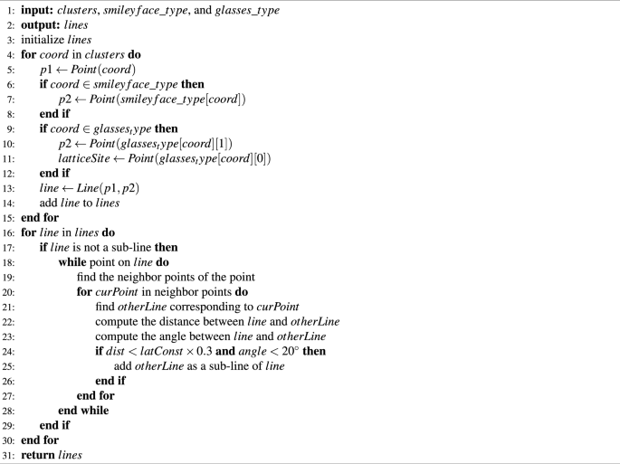
The pseudocode for constructing SIA line components is shown in Algorithm 5.
SIA Line Component Construction Method
Further description of the pseudocode is provided below:
(a) clusters stores all clusters in dictionary form, with the key being the cluster number and the value being the indices of all defects contained in that cluster in the defect array. Smileyface_type and glasses_type clusters also store all defects in dictionary form, with the key being one defect’s index and the value being another or two other defects’ indices. The defect points in each cluster are traversed sequentially, and if the current defect point is in smileyface_type and glasses_type clusters, then the index of the corresponding defect point is found, and the two points are connected as a line, which is then added to the lines array.
(b) For each line in the lines array, if the current line is not a sub line (i.e., it does not contain the “parent” parameter), all points on the points parameter of the current line are traversed. Using the nearest neighbor algorithm K-D tree, other points in the neighborhood of each point are found, and the line to which these points belong is located. The distance and angle between the current line and these lines are calculated. If the distance is less than 0.3 times the lattice constant and the angle is less than 20\(^\circ\), the lines can be merged within the allowable spatial error, and these lines become sub lines of the current line.
This paper takes a cluster containing 13 defect points as an example, as shown in Fig. 16. After calculating the defect list, the smileyface_type and glasses_type of the cluster are {P1:(P0, P2), P4:(P3, P5), P7:(P6, P8)}, {P10:P9, P11:P12}. Using the component construction method, these defects are connected into five lines. When the neighboring point P11 of P2 is found, the line L4 containing P11 is located, and the distance and angle between L0 and L4 are calculated. If the merging rules are satisfied, the adjacent overlapping lines and collinear points are merged, and the cluster is eventually represented as a cluster of three lines, yielding the componentized information for this cluster.

Construction of SIA line assemblies.
Defect cluster configuration identification algorithm
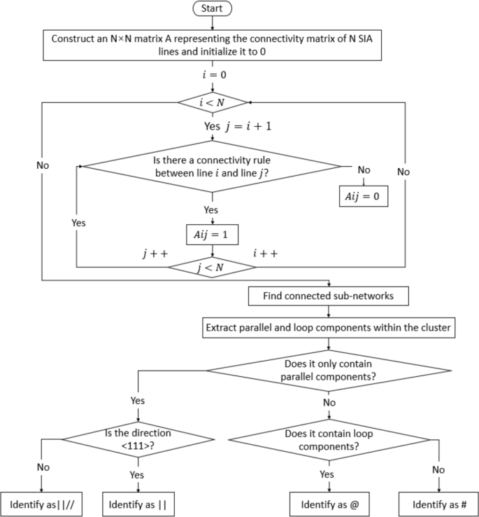
For the multiple SIA lines within the cluster, it is necessary to further clarify the positional relationship between them to identify the detailed configuration of the defects. This paper establishes an automatic identification mechanism based on the typical features of clustered configurations, as shown in Fig. 17.
Algorithm steps for defect cluster configuration identification.
First, an \(N \times N\) adjacency matrix A is constructed to represent a cluster with N SIA lines. The number of rows and columns of the matrix corresponds to the number of SIA lines, and the matrix’s values indicate the positional relationship between the i-th and j-th SIA lines, as determined by the connectivity rules of the graph. If the i-th and j-th SIA lines satisfy the connectivity rules, then the value \(a_{ij} = 1\); otherwise, \(a_{ij} = 0\). The connectivity rules are defined as follows:
For parallel components, \(a_{ij}\) is defined as equation 11:
$$\begin{aligned} a_{ij} = {\left\{ \begin{array}{ll} 1, & \text {if } d \le 1N \text { and } \theta \approx 0, \\ 0, & \text {otherwise}. \end{array}\right. } \end{aligned}$$
(11)
That is, if the shortest distance between two SIA lines is less than or equal to the nearest neighbor distance value \(\sqrt{3}/2\, c_0\) and the angle is close to \(0^\circ\), then the two SIA lines are considered parallel components. For ring components, \(a_{ij}\) is defined as equation 12:
$$\begin{aligned} a_{ij} = {\left\{ \begin{array}{ll} 1, & \text {if } d = 1 \text { NN or } 3 \text { NN}, \text { and } \theta \approx 60^\circ \text { or } 90^\circ , \\ 0, & \text {otherwise}. \end{array}\right. } \end{aligned}$$
(12)
That is, if the shortest distance between two SIA lines is equal to the nearest neighbor or third-nearest neighbor distance value \(\left( \sqrt{2}\, c_0 \right)\), and the angle is approximately \(60^\circ\) or \(90^\circ\), then they are considered ring components. The two valid distance and angle values account for the two possible configurations of ring components due to different spatial arrangements in 3D space.
Based on the above rules, a matrix is calculated, and the connected components of the graph represented by the matrix are identified, as illustrated in Fig. 18. In defect clusters, a large number of defect atoms form numerous SIA lines, resulting in a high-order matrix with many zero elements, forming a sparse matrix. Storing this matrix directly would waste a significant amount of storage space. Therefore, to save space, the sparse matrix needs to be compressed before storing and calculating the graph’s connectivity.

Searching for connected components of a sparse matrix.
Compressed Sparse Row (CSR) is an effective method for storing compressed sparse matrices49. This storage structure includes three arrays: data, indices, and indptr. data stores the values corresponding to each non-zero element; indices stores the column index of each element; and indptr stores the number of non-zero elements in the previous row for each row, starting from 0. This storage format effectively compresses sparse matrices and allows for more efficient searching for connected components later.
Each SIA line is treated as a node, and their neighboring relationships are treated as edges. According to the definitions of parallel and ring components, it is determined whether they are connected. For parallel components, if two neighboring nodes represent parallel SIA lines, an edge is added between them. For ring components, if the neighboring nodes represent SIA lines that meet the given distance and angle conditions (approximately \(60^\circ\) or \(90^\circ\)), an edge is added. Then, connected components are found using graph theory algorithms, and the connected components are represented as parallel or ring components, as shown in Fig. 19.

Connected components are represented as parallel components or ring components.
The pseudocode for the connected component search algorithm within the cluster is as Algorithm 6.
Construction Method for SIA Line Components
A detailed explanation of the pseudocode is provided below:
(a) The adjacency matrix A is constructed based on the neighboring connections between components and stored in CSR format, allowing queries to find all components connected to each component.
(b) All components’ collection numbers are initialized using their component numbers. In the initial state, each component is treated as a separate collection.
(c) Traverse all components based on the component number. If the assembly number of the set that the current component belongs to is different from the component number, it indicates that this component belongs to the same set as other components that have already been traversed and will not be processed further. Otherwise, attempt to use this component as an entry point to find all components that belong to the same set.
(d) Use a breadth-first search algorithm to initialize the component queue with the current component. While the queue is not empty, it indicates that there are still unmarked components in the current set. Remove a component from the front of the queue, mark its assembly number, and query the adjacency matrix A to obtain all components that are connected to it. If any of these components have already been marked, then mark this set as a ring component, and send all unmarked components into the component queue. Once the queue is empty, it can be determined that all components in the current set have been marked. Based on the numbers of all components in the set, the components are classified as parallel components, ring components, or isolated components, and this set is added to the assembly result list.
(e) After completing the marking of assembly numbers for all components, return the assembly result list.
By searching for connected components, parallel components and ring components can be found. However, there may be some components that do not have specific configurations, which are neither parallel components nor ring components. These are mainly transient structures caused by thermal vibrations, which will transition to stable parallel or ring structures at room temperature.
Regarding the structural characteristics of parallel components and ring components, this paper uses different symbols to visually represent several configurations that defects may exist in, including stable configurations with only one type of defect and metastable configurations composed of multiple components, as specifically described in Table 10.
Analysis and verification of defect statistics
This paper uses the MISA-MD simulation dataset of cascade collision data for BCC pure iron for experimental analysis and verification, outputting atomic position coordinate information every 1000 time steps. A detailed description of the dataset can be found in Table 11.
This paper employs the dual-pointer lattice filling method to count the number of Frenkel defect pairs under different PKA energies and different PKA directions when the MISA-MD simulation reaches a stable state (the 41,000th time step) and compares the results with those obtained from OVITO (the Open Visualization Tool, version 3.10.2; https://www.ovito.org/)52. The results are consistent, as shown in Table 12. Compared to the W-S unit cell method, the method used in this paper reduces the storage space occupied by unnecessary arrays while ensuring the correctness of the results.
Using the dual-pointer lattice filling method, the number of defect pairs at each time step under energies of 10 keV, 20 keV, 30 keV, and 50 keV, with incident directions of [122], [135], and [235], is counted, as shown in Fig. 20a,b, Fig. 20c,d, respectively.
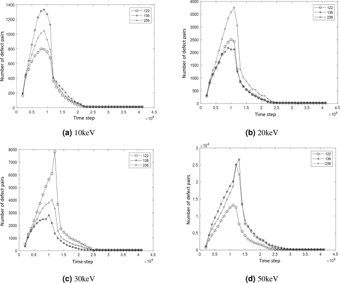
Curve of Defect Quantity Variation with PKA Directions at different energy.
From the curves of defect pair quantity changes, it can be seen that regardless of the energy or direction in the simulation, the trend of defect pair quantity generally follows a similar pattern. Initially, as simulation time increases, the quantity rapidly increases, reaches a certain peak, and then gradually decreases, stabilizing at around the 23,000th simulation time step. The peak time, stable time, and stable quantity of Frenkel defect pairs are consistent with the trends shown in OVITO, and the final surviving quantity of Frenkel defect pairs aligns with the classical NRT model.


