Thermodynamically consistent machine learning model for excess Gibbs energy

HANNA architecture

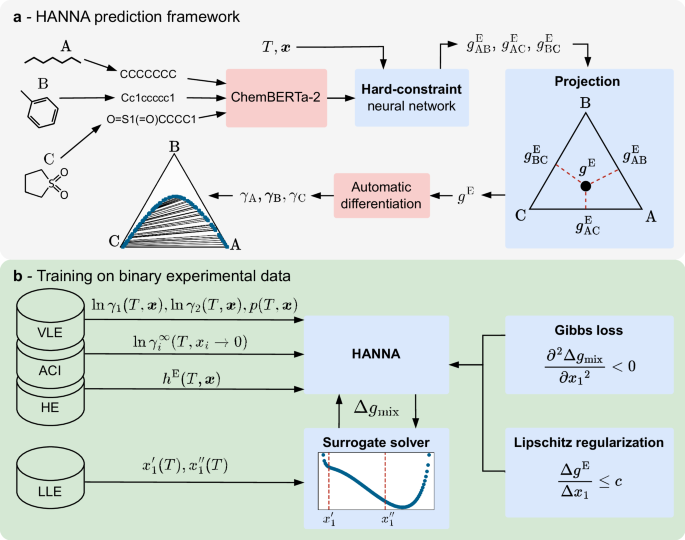
The algorithm in Box 1 explains the forward pass of the HANNA architecture, starting with the temperature, the composition, and the molecular embeddings of an arbitrary N-component mixture of interest as input and providing predictions for the activity coefficients of the N components and the scaled molar excess Gibbs energy in the mixture as output.

The input of HANNA contains the numerical molecular embeddings e_i of the N components that make up the mixture to be modeled, summarized in E = [e₁, …, e_N], which are calculated individually with the transformer-based model ChemBERTa-2 from the respective component’s SMILES (canonized with RDKit⁴⁹). We use the 77M-MTR variant of ChemBERTa-2 from Hugging Face⁴² with a slightly corrected tokenizer³². Additionally, HANNA requires the temperature T and the mole fractions x₁, …, x_N−1 of N − 1 components as input. The HANNA architecture comprises three feed-forward neural networks (FFNNs), namely, the EmbeddingNetwork, the MixtureNetwork, and the PropertyNetwork. The EmbeddingNetwork consists of one layer, while the other two networks consist of two layers. In all cases, we use the Sigmoid Linear Unit activation function.

All layers are modified linear layers with 96 nodes (except for the input layer of the MixtureNetwork, which consists of 98 nodes, as the temperature and the projected mole fraction of the respective component are concatenated to the output of the EmbeddingNetwork) to which a Lipschitz regularization (cf. section “Training of HANNA”) is applied. HANNA computes the molar excess Gibbs energy for the N-component mixture of interest through a geometric projection from the binary subsystems^{40,41,50,51,52}. For this purpose, the mole fractions of the N-component mixture are projected onto all N(N−1)/2 binary subsystems (cf. loop in step 6 of the algorithm in Box 1). In this work, we use the Muggianu projection³³, which, unlike other projection methods, does not exhibit singular points at infinite dilution^53,54. The projected mole fractions \({X}_{i}^{\,(ij)}\) and \({X}_{j}^{\,(ij)}\) in the binary subsystem i–j are given by:

whereby \({\widetilde{x}}_{i}\) and \({\widetilde{x}}_{j}\) are the corrected mole fractions of component i and j, respectively (cf. below). The projection strictly fulfills the summation condition in each binary subsystem, i.e., \({X}_{i}^{\,(ij)}+{X}_{j}^{\,(ij)}=1\). Furthermore, if a binary mixture is studied, the projected mole fractions reduce to the corrected mole fractions, i.e., \({X}_{i}^{\,(ij)}={\widetilde{x}}_{i}\) and \({X}_{j}^{\,(ij)}={\widetilde{x}}_{j}\), ensuring a consistent transition of the HANNA predictions going from a binary to a multi-component mixture. In contrast to the original publication³³, we correct the original mole fractions x_i in the N-component mixture before the projection as follows (cf. steps 4 and 5 of the algorithm in Box 1):

With this correction, we lump identical components, indicated by a component similarity score R_ij = 1, into a single component, thereby ensuring that, e.g., for a system of three components A, B, and C, where B is identical to C, the exact same results are obtained as for the binary system of A and B (when accounting for the lumped mole fractions). To compute the component similarity score R_ij, we apply the radial basis function (RBF) on pairs of the refined molecular embeddings. By setting the hyperparameter β of the RBF to the high value of 100, we ensure that only extremely similar components result in a similarity score of R_ij = 1, so only components that we consider truly identical are lumped together.

Finally, the molar excess Gibbs energy g^E of the N-component mixture is calculated as follows⁴¹:

where \({g}_{ij}^{{{{\rm{E}}}}}\) is the molar excess Gibbs energy of the binary subsystem i–j and q_ij is the learned binary interaction between component i and j in the respective binary subsystem. q_ij is calculated using a deep set architecture⁵⁵ including a summation aggregation (cf. step 6d of the algorithm in Box 1) to ensure the permutation invariance of the predicted molar excess Gibbs energy, i.e., to ensure that the order of the components in the input of HANNA does not influence its results. For technical reasons, namely, to prevent divisions by zero in Eq. (3) if one of the projected mole fractions approaches zero, we directly predict the binary interaction term q_ij with HANNA for each binary subsystem in the projected space (cf. step 6e of the algorithm in Box 1). Here, again, the component similarity score R_ij is used, ensuring thermodynamically sound predictions by enforcing q_ij = 0 and, ultimately, \({g}_{ij}^{{{{\rm{E}}}}}=0\) for identical components i and j. Using the Autograd functionality of PyTorch⁵⁶, the activity coefficients for all N components are finally derived from g^E of the N-component mixture (cf. steps 8 and 9 of the algorithm in Box 1), ensuring strict Gibbs-Duhem consistency⁵⁷.

Data

The experimental data used to train and evaluate HANNA in this work were taken from the 2025 version of the DDB³⁴. Data points labeled as poor quality by the DDB’s internal criteria were excluded. Furthermore, only components for which a canonical SMILES string could be generated with RDKit⁴⁹ using mol-files from the DDB were considered. Table 2 gives an overview of the final datasets of the different data types for binary, ternary, and quaternary systems. A detailed description of each data type is given below.

Two types of experimental VLE data were used in this work: On the one hand, we considered data points in the DDB³⁴ that contain all information on temperature, pressure, as well as liquid and vapor phase compositions. These are labeled as TPXY data. From the TPXY data, activity coefficients for all components i were calculated with the extended Raoult’s law:

Here, γ_i is the activity coefficient of component i normalized according to Raoult’s law in the mixture, x_i and y_i are the mole fractions of component i in the liquid and vapor phase in VLE, respectively, p denotes the total pressure, and \({p}_{i}^{{{{\rm{s}}}}}\) is the pure-component vapor pressure of i at the same temperature as the VLE data. The pure-component vapor pressures were computed using the Antoine equation with coefficients from the DDB³⁴. On the other hand, we used VLE data that does not include information on the composition of the vapor phase. Consequently, these are labeled as TPX data. Because activity coefficients cannot be calculated for the TPX data, we use total pressure as the training objective for those data points. By using extended Raoult’s law for all VLE data points in our work, we assume that the vapor phase can be treated as an ideal gas mixture and that the pressure dependence of the chemical potential in the liquid phase can be neglected. To justify these assumptions, all TPXY and TPX data points with pressures higher than 10 bar were excluded.

Activity coefficients at infinite dilution \({\gamma }_{i}^{\infty }\) normalized according to Raoult’s law, called “ACI” throughout this work, were considered for binary and ternary mixtures. For binary mixtures, i.e., with pure solvents, these data could be used directly. For the activity coefficients at infinite dilution in mixed solvents, we observed several errors in the DDB, mostly interchanged solvent labels, so that these data had to be curated prior to use. Our detailed data curation protocol is described in the following: For each ternary ACI system reported at temperature T_ACI, we compared the reported logarithmic activity coefficients at infinite dilution \(\ln{\gamma }_{3}^{\infty }\) at the pure-solvent endpoints (i.e., x₁ = 0 or x₂ = 0) with those of the same solute in the corresponding pure solvents from the binary ACI data at temperatures within ±5 K of T_ACI. Systems for which no such binary reference data were available, or for which the absolute deviation exceeded a value of 0.1, were excluded. Only the remaining mixed-solvent data points (x₁ ≠ 0 and x₂ ≠ 0) of the retained systems were included in the final dataset.

The LLE data in the DDB contains information on the temperature T and the mole fractions in the coexisting phases \({x}_{i}^{{\prime} }\) and \({x}_{i}^{{\prime\prime} }\) (and \({x}_{i}^{{\prime\prime} {\prime} }\) in the case of a three-phase equilibrium). Here, data for binary, ternary, and quaternary mixtures were considered. For binary data, we followed the notation of the DDB and defined the phase compositions such that \({x}_{1}^{{\prime} }\) is always the phase composition with the lower value, i.e., \({x}_{1}^{{\prime\prime} } > {x}_{1}^{{\prime} }\) always holds, which is important for training the surrogate solver, cf. section “Surrogate LLE solver”. Only for roughly a quarter of the LLE data points in the DDB all phase compositions are reported at the specified temperature. For the remaining data points, only the composition of one phase is available. Nonetheless, we included these data points in our dataset. Because HANNA does not consider the pressure dependence of the excess Gibbs energy and thus the activity coefficients, we excluded all LLE data points with pressures above 50 bar.

Finally, we also extracted experimental data for the excess enthalpies h^E of binary and ternary mixtures from the DDB. Each data point consists of the temperature T, the mole fraction x₁, and the excess enthalpy h^E.

Data splitting and scaling

Following a cross-validation approach, we randomly split the datasets for binary mixtures system-wise into 10 folds, each representing a mutually exclusive test set of 10% of the binary systems. A stratified split strategy was employed, such that the share of each data type is roughly equal for all folds. The remaining data (90% of the systems) of each fold were again split system-wise into a training set (90%) and a validation set (10%). In the data splits, all types of data for a particular system were put exclusively within a single set; for instance, if LLE data for a particular system were in the test set, all TPXY, TPX, ACI, and HE data for this system were also in the test set. This strategy enabled the use of all available data as unseen test data for the evaluation of HANNA.

Furthermore, an additional data split was carried out, where 95% of the binary systems were used in the training set and 5% in the validation set (i.e., no test set was withheld). This split, denoted as “full data split” in the following, was used to train the model that was subsequently evaluated on the data for ternary and quaternary systems and is also deployed as the “final model” with this work.

The molecular embeddings from ChemBERTa-2, as well as the temperature, were scaled using the scikit-learn⁵⁸ StandardScaler(). Individual scalers were fitted to each training dataset to prevent any information leakage.

Surrogate LLE solver

From the binary TPXY data points, activity coefficients can be calculated directly using the extended Raoult’s law, cf. Eq. (4). Hence, the training of HANNA on these data is straightforward using a loss function for the predicted activity coefficients, cf. section “Training of HANNA”. In contrast, it is not possible to explicitly calculate activity coefficients from the binary experimental LLE data. Using HANNA, one could obtain phase compositions for a given system and state point using iterative solvers³⁵ and compare them to experimental data. However, integrating iterative solvers into a deep learning framework is tedious because gradients are not easily trackable and, moreover, it would significantly slow down the training process. To overcome this, we developed a differentiable surrogate solver to estimate the binary LLE phase compositions resulting from the activity coefficients predicted by HANNA. This surrogate solver is realized by an FFNN that mimics the CEM^37,38,39 and maps a discretized graph of the scaled molar Gibbs energy of mixing

onto the compositions of the two coexisting liquid phases \({x}_{1}^{{\prime} }\) and \({x}_{1}^{{\prime\prime} }\). During the training of HANNA, the surrogate solver allows the model to directly learn from experimental LLE data while maintaining full compatibility with gradient-based optimization. The architecture and training process of the surrogate solver are described in the following.

As input, the surrogate solver gets a vector of Δg_mix/(RT) values calculated with HANNA at 101 uniformly spaced discrete compositions from x₁ = 0 to x₁ = 1 mol mol⁻¹ at constant temperature T. The Δg_mix/(RT) values from HANNA are then processed through three fully connected layers with a hidden size of 64, each followed by the Rectified Linear Unit (ReLU) activation function. The output layer yields two values that correspond to \({x}_{1}^{{\prime} }\) and \({x}_{1}^{{\prime\prime} }\) (we always define \({x}_{1}^{{\prime} }\) as the phase composition with the lower value, cf. section “Data”), which are subsequently processed through a sigmoid function to constrain the mole fractions between 0 and 1. To align with the demand of thermodynamic consistency of the model, the surrogate solver must be permutation-equivariant with respect to the order of the molecules in the input, i.e., if the discretized Gibbs energy of mixing is given in reverse order, it must yield \(1-{x}_{1}^{{\prime\prime} }\) and \(1-{x}_{1}^{{\prime} }\). To enforce this, upon calling the forward function of the surrogate solver with a discretized Δg_mix/(RT) vector, the phase compositions are calculated twice, both from the original vector and the reversed vector. The two values obtained for \({x}_{1}^{{\prime} }\) and \({x}_{1}^{{\prime\prime} }\) are then averaged. Besides guaranteeing permutation-equivariance, this procedure also prevents any bias in the order of the training data from negatively impacting the training.

The surrogate solver was trained only on synthetic data, namely, predictions of Δg_mix/(RT) obtained with mod. UNIFAC. More specifically, for every experimental LLE data point in our dataset within the mod. UNIFAC horizon, we calculated Δg_mix/(RT) for the 101 discrete uniformly spaced compositions at the temperature of the respective data point with mod. UNIFAC. We then used the CEM to determine the corresponding phase compositions, which served as the training objective of our surrogate solver. If no phase split was found, the data point was dropped. We used the same system-wise split as for the experimental data (cf. section “Data splitting and scaling”) to split the synthetic surrogate solver data into training, validation, and test sets. This prevents information leakage through the surrogate solver when training HANNA. We trained separate surrogate solvers for each fold on the synthetic Δg_mix/(RT) values of the corresponding LLE training data. The surrogate solvers were trained for 200 epochs, using the Adam optimizer with the MSE loss and the OneCycleLR scheduler (max_lr = 0.01), and the best model was selected based on the validation loss (the validation dataset was generated in the same manner as the training set). Results of the surrogate solver training are provided in the Supplementary Note 1, along with an example of its functionality given in Supplementary Fig. 1.

Training of HANNA

HANNA was trained by minimizing the total loss \({{{{\mathcal{L}}}}}_{{{{\rm{total}}}}}\), defined as:

where N_b is the batch size, \({{{{\mathcal{L}}}}}_{{{{\rm{TPXY}}}}},{{{{\mathcal{L}}}}}_{{{{\rm{TPX}}}}},{{{{\mathcal{L}}}}}_{{{{\rm{ACI}}}}},{{{{\mathcal{L}}}}}_{{{{\rm{LLE}}}}},{{{{\mathcal{L}}}}}_{{{{\rm{HE}}}}}\) are the individual data losses, \({{{{\mathcal{L}}}}}_{{{{\rm{Gibbs}}}}}\) is the Gibbs loss, \({{{{\mathcal{L}}}}}_{{{{\rm{Lips}}}}}\) is the Lipschitz regularization, and w_TPX, w_LLE, w_HE, w_Gibbs, w_Lips are the corresponding weight factors that were determined in a hyperparameter grid search, cf. Supplementary Note 2 for details.

In the individual data losses, we use the SmoothL1Loss() loss function from PyTorch⁵⁶, which is less sensitive to outliers than the mean squared error loss. The parameter β in the SmoothL1Loss() function, which controls the transition between the mean absolute and mean squared error, was empirically set for each data type individually.

\({{{{\mathcal{L}}}}}_{{{{\rm{TPXY}}}}}\) penalizes the average deviation of the two logarithmic activity coefficients predicted with HANNA from the respective experimental values derived from the TPXY data for the binary systems from the training set:

where N_TPXY is the number of TPXY data points in the training batch. Similarly, \({{{{\mathcal{L}}}}}_{{{{\rm{ACI}}}}}\) takes into account errors in the prediction of the activity coefficients at infinite dilution \(\ln{\gamma }_{i}^{\infty }\) for the binary systems from the training set:

where N_ACI is the number of ACI data points in the batch. The factor \(\frac{1}{2}\) takes into account that in \({{{{\mathcal{L}}}}}_{{{{\rm{ACI}}}}}\), only the activity coefficient at infinite dilution contributes to the loss calculation, whereas in \({{{{\mathcal{L}}}}}_{{{{\rm{TPXY}}}}}\), the errors of both activity coefficients of the binary mixture are averaged before contributing to the loss. \({{{{\mathcal{L}}}}}_{{{{\rm{TPX}}}}}\) accounts for the difference of the predicted logarithmic total pressures to the experimental ones on the N_TPX data points:

The predicted logarithmic total pressures are calculated from the predicted activity coefficients and the pure component vapor pressures:

\({{{{\mathcal{L}}}}}_{{{{\rm{LLE}}}}}\) denotes the loss between the LLE phase compositions in mole fractions predicted by HANNA and the experimental values in the batch obtained through

where N_LLE is the number of LLE data points in the batch and m_k ∈ {0, 1} is a binary mask that indicates if the respective data point is considered or not (cf. below for details). To obtain the predicted phase compositions \({x}_{1,{{{\rm{pred}}}}}^{{\prime} },{x}_{1,{{{\rm{pred}}}}}^{{\prime\prime} }\) for a data point during training, the pre-trained surrogate solver (cf. section “Surrogate LLE solver”) is provided with the discretized molar Gibbs energy of mixing curve for the respective system and temperature. For the LLE data points with only one available phase composition, the loss term in Eq. (11) is calculated only on this phase composition. Since the surrogate solver is only trained on positive samples (i.e., binary LLE systems at state points with a miscibility gap) and cannot identify systems without miscibility gap, it will also falsely predict a phase split for a Δg_mix that does not fulfill the necessary condition for a phase split, which states

i.e., the second derivative of Δg_mix is negative somewhere in the composition space. This is unphysical and could potentially negatively impact the training process. Therefore, during the training, we account for the LLE loss of binary systems only if the necessary condition in Eq. (12) is true for at least one discretized composition; this is reflected in Eq. (11) through the binary mask m_k, where m_k = 1 for data points that exhibit an LLE and m_k = 0 for those that do not. The required second derivatives of Δg_mix were calculated by automatic differentiation. \({{{{\mathcal{L}}}}}_{{{{\rm{HE}}}}}\) describes the loss on the N_HE excess enthalpy data points:

The predicted excess enthalpy is calculated using³⁵

The factor 1/s_T in Eq. (14) follows from the chain rule because HANNA uses the scaled temperature T^* = (T−μ_T)/s_T as input.

The \({{{{\mathcal{L}}}}}_{{{{\rm{LLE}}}}}\) described above alone does not penalize false negative LLE predictions. If HANNA fails to predict a liquid–liquid phase split, the necessary condition in Eq. (12) is not fulfilled, and the binary mask is m_k = 0, cf. Eq. (11). To provide a learning incentive towards a correct detection of these phase splits, the additional loss term \({{{{\mathcal{L}}}}}_{{{{\rm{Gibbs}}}}}\) was introduced:

Here,

is the second derivative of the molar Gibbs energy of mixing for data point k from the LLE training set evaluated at the composition d on the discretized grid of Δg_mix. Eq. (15) identifies the minimum of the second derivative of Δg_mix within the discretized composition space for each LLE training data point. If this minimum is negative, a miscibility gap is predicted by the model (cf. Eq. (12)) and the Gibbs loss is zero. Note that in this case (m_k = 1), the deviation to experimental data is accounted for by \({{{{\mathcal{L}}}}}_{{{{\rm{LLE}}}}}\). If the minimum is positive, the miscibility gap is not identified by HANNA, and, consequently, the model is penalized by adding the respective value of S_k to the total loss.

Besides the data losses and the Gibbs loss, \({{{{\mathcal{L}}}}}_{{{{\rm{Lips}}}}}\) is included in the total loss function as a Lipschitz regularization term, controlling the Lipschitz constant of HANNA. Generally, the Lipschitz constant (c ≥ 0) in the 2-norm is defined as

and provides an upper bound for the change of a function from f(x₀) to f(x₁) by changing the function input from x₀ to x₁; it is, therefore, a proxy for the smoothness of a function. For fully connected neural networks with L layers, a loose upper bound

is obtained by the product of the spectral norms ∥W_l∥₂ of the weight matrices of each layer l, if the Lipschitz constants of the activation functions are neglected⁵⁹. For HANNA, the influence of the summation of the two mixture embeddings (cf. step 6d of the algorithm in Box 1) on the total Lipschitz constant is also neglected, since it does not contain any learnable parameters. The spectral 2-norm ∥W_l∥₂, in turn, equals the maximum singular value \({\sigma }_{\max }({{{{\bf{W}}}}}_{l})\) of the weight matrix W_l⁶⁰.

Following the approach from ref. ⁵⁹, all networks of HANNA are realized as modified linear layers with learnable Lipschitz constants \({c}_{l}^{*}\). In these layers, the raw weight matrices W_raw are first normalized using the maximum singular value \({\sigma }_{\max }({{{{\bf{W}}}}}_{l,{{{\rm{raw}}}}})\) (such that their Lipschitz constant equals one) and then scaled using the learnable Lipschitz constants:

These scaled weight matrices are then used in the forward function of the modified layers as a drop-in replacement of the raw weight matrices. For computational efficiency, we approximate \({\sigma }_{\max }({{{{\bf{W}}}}}_{l,{{{\rm{raw}}}}})\) with a power iteration method using two iterations⁶⁰. The Lipschitz regularization term used in the total loss function, cf. Eq. (6), is calculated via⁵⁹

by multiplying the total Lipschitz constants of the networks (given by the product of the layer-wise learned constants of all L layers in the model and ignoring other factors, cf. above). The softplus transformation of \({c}_{l}^{*}\) avoids infeasible negative Lipschitz constants⁵⁹. The hyperparameter w_Lips, cf. Eq. (6), can be used to control the learnable Lipschitz constants of the network, i.e., higher values of w_Lips lead to lower Lipschitz constants and vice versa. For the model variants in the grid search with w_Lips = 0, we employed an L2-regularization instead to prevent exploding parameters.

The HANNA models for this work were trained for 200 epochs using a batch size of 512, the AdamW optimizer, and the OneCycleLR scheduler (max_lr = 0.01) from PyTorch. The best epoch was selected based on the weighted sum of the data losses (\({{{{\mathcal{L}}}}}_{{{{\rm{TPXY}}}}},{{{{\mathcal{L}}}}}_{{{{\rm{TPX}}}}},{{{{\mathcal{L}}}}}_{{{{\rm{ACI}}}}},{{{{\mathcal{L}}}}}_{{{{\rm{LLE}}}}}\), and \({{{{\mathcal{L}}}}}_{{{{\rm{HE}}}}}\)) on the respective validation set, whereby only models that were trained for at least 50 epochs were considered.

After determining the optimal hyperparameters through a grid search (cf. Supplementary Note 2), we trained an ensemble of 10 models (starting from different weight initializations) for each data fold (cf. section “Data splitting and scaling”). Additionally, we trained such an ensemble for the full data split; this model is also published as the final model along with this work. Training was carried out on NVIDIA A30 GPUs; a typical training run of a single HANNA model (200 epochs) required approximately 20 h.

Evaluation of HANNA

For the systematic evaluation of HANNA and the benchmark models, absolute deviations ϵ between the predicted and the experimental values for each data point in the considered test set were calculated.

For each TPXY data point, a mean absolute deviation of the logarithmic activity coefficients of all components i in the test mixture at the respective temperature T and composition x was calculated:

Here, N is the number of components in the mixture (N = 2 for binary, N = 3 for ternary, N = 4 for quaternary mixtures).

To evaluate the model performance on the TPX data points, the absolute deviations in the logarithmic total pressures were calculated:

For each ACI data point, i.e., activity coefficients at infinite dilution in pure or in mixed solvents, only the logarithmic activity coefficient of the infinitely diluted solute i in the solvent(s) was considered for error calculation:

The LLE predictions were evaluated through the mean absolute deviation of the phase compositions in mole fractions \({x}_{i}^{{\prime} }\) and \({x}_{i}^{{\prime\prime} }\) (and \({x}_{i}^{{\prime\prime} {\prime} }\) for three-phase equilibria) of all components i in the mixture:

Here, π denotes the number of liquid phases. For the HE data, the absolute deviation of the excess enthalpies in kJ mol⁻¹ was used as evaluation metric:

From the data point-wise error scores described above, system-wise mean absolute error MAE_sys scores were calculated by averaging over all data points (at all temperatures and compositions) for each binary, ternary, or quaternary system. The system-wise error scores are favorable as they are independent of the number of available data points for a particular system and do not over-emphasize systems with many data points, such as (ethanol + water). Therefore, they are more suitable to evaluate the performance of the models to generalize over unseen systems and components.

The HANNA predictions shown in the evaluation of this work were obtained using ensembles of 10 individual models. For the binary data, we used the 10 independently trained ensembles and evaluated them on their respective test set. For the multi-component data, the final model, i.e., the ensemble trained on the full data split, was used.