
Preliminaries
Traffic network
As shown in Fig. 2, the corresponding road network topology is generated according to the road connection relationship between each sensor in the actual road network, which is represented by \(G=\left(V,E,A\right)\), where \(V=\left\{{v}_{1},{v}_{2},\dots ,{v}_{N}\right\}\) represents the set of all nodes (road sensors) in the entire road network, and \(N\) represents the number of nodes. \(E\) is a set of edges representing the connectivity between nodes. If there are two nodes connected by a road, then there is an edge in \(G\) connecting the two nodes. \(A\in {R}^{N\times N}\) is the adjacency matrix, \({a}_{ij}\) is an element in \(A\), which represents the spatial connection state between node \({v}_{i}\) and node \({v}_{j}\). If there exist \({v}_{i},{v}_{j}\in V\) and \(\left({v}_{i},{v}_{j}\right)\in E\), then the value of \({a}_{ij}\) is 1, otherwise it is zero.

Road network generates spatial topography.
Construction of time characteristics
The time characteristics of all nodes in the topological graph \(G\) are represented by \(X\in {R}^{N\times L\times F}\), where \(L\) denotes the total length of time series of each node, \(F\) denotes the number of types of characteristics of nodes. The process of traffic flow prediction can be described by Eq. (1):
$$\begin{array}{c}\left({X}_{t+1},{X}_{t+2},\dots ,{X}_{t+{T}{\prime}}\right)=F\left[\left({X}_{t-T+1},{X}_{t-T+2},\dots ,{X}_{t}\right);G\right],\end{array}$$
(1)
where \(t\) denotes a moment, \(T\) is the length of historical traffic data, and \(T{\prime}\) is the length of future traffic data to be predicted. Given continuous time steps \(\left({X}_{t-T+1},{X}_{t-T+2},\dots ,{X}_{t}\right)\) and topological graph \(G\), by training a model \(\mathcal{F}\), we can predict the future \(T{\prime}\) continuous time steps \(\left({X}_{t+1},{X}_{t+2},\dots ,{X}_{t+{T}{\prime}}\right)\).
STCMFA model
Figure 3 shows the overall framework of STCMFA, which is mainly composed of input layer (Multi-Layer Perceptron, MLP1), GCN, aggregation layer, TS-MFA module, and output layer (MLP2). We will describe each module of STCMFA in detail below.

The overall structure of STCMFA.
Graph convolutional network
The spectral graph theory studies the influence of the eigenvalues and corresponding eigenvectors of the Laplacian matrix of the graph on the topological properties of the graph42. In spectral analysis, for a graph \(G\), its Laplacian matrix can be expressed as:
$$\begin{array}{c}L={I}_{N}-{D}^{-\frac{1}{2}}A{D}^{-\frac{1}{2}},\end{array}$$
(2)
where \(A\) is an adjacency matrix, and the degree matrix \(D\in {R}^{N\times N}\) is a diagonal matrix, defined as \({D}_{ii}=\sum_{j}{A}_{ij}\). \({I}_{N}\) is a unit matrix of size \(N\times N\), \(L\in {R}^{N\times N}\). The eigenvalue decomposition of the Laplacian matrix is obtained:
$$\begin{array}{c}L=U\Lambda {U}^{T},\end{array}$$
(3)
$$\begin{array}{c}\Lambda =diag\left(\left[{\lambda }_{0},{\lambda }_{1},\dots ,{\lambda }_{N-1}\right]\right)\in {R}^{N\times N}.\end{array}$$
(4)
In Eq. (3), \(\Lambda \) is a diagonal matrix composed of eigenvalues of \(L\), as shown in Eq. (4). \(U=\left\{{u}_{1},{u}_{2},\dots ,{u}_{N}\right\}\) is the eigenvector of \(L\).
We set \(x={X}_{t}\in {R}^{N}\) as the signal of the whole graph, and define the Fourier transform of the signal as \(\widehat{x}={U}^{T}x\). The signal \(x\) on \(G\) can be filtered by the convolution kernel \({g}_{\theta }\):
$$\begin{array}{c}{g}_{\theta }*Gx=U{g}_{\theta }\left(\Lambda \right){U}^{T}x,\end{array}$$
(5)
where \(*G\) denotes the graph convolutional operation. To speed up the solution of the characteristic matrix, we use the Chebyshev polynomial to approximate the eigenvalue matrix. The Chebyshev polynomials can be expressed by Eq. (6):
$$\begin{array}{c}{g}_{\theta }\left(\Lambda \right)=\sum_{k=0}^{K-1}{\theta }_{k}{T}_{k}\left(\widetilde{\Lambda }\right),\end{array}$$
(6)
where \(\theta \in {R}^{K}\) is the vector of Chebyshev polynomial coefficients, and \({T}_{k}\left(\widetilde{\Lambda }\right)\in {R}^{N\times N}\) is the Chebyshev polynomial of order \(K\) of \(\widetilde{\Lambda }\). And \(\widetilde{\Lambda }=\frac{2}{{\lambda }_{max}}\Lambda -{I}_{N}\), that is, the eigenvalue diagonal matrix after the range normalization, \({\lambda }_{max}\) is the maximum value of the eigenvalue. The recurrence formula of Chebyshev polynomials of order \(k\) is \({T}_{k}=2x{T}_{k-1}\left(x\right)-{T}_{k-2}\left(x\right)\). The first two terms of the recurrence equation are \({T}_{0}\left(x\right)=1, {T}_{1}\left(x\right)=x\). The graph convolutional operation after Chebyshev approximation can be defined as the following equation:
$$\begin{array}{c}{g}_{\theta }*Gx=U{g}_{\theta }\left(\Lambda \right){U}^{T}x=U\left(\sum_{k=0}^{K-1}{\theta }_{k}{T}_{k}\left(\widetilde{\Lambda }\right)\right){U}^{T}x\approx \sum_{k=0}^{K-1}{\theta }_{k}{T}_{k}\left(\widetilde{L}\right)x,\end{array}$$
(7)
where \(\widetilde{L}=\frac{2}{{\lambda }_{max}}L-{I}_{N}\). Equation (7) can be understood as extracting the information of 0 to \(K-1\) neighbors around each node in the topology graph through the convolution kernel \({g}_{\theta }\). After each graph convolutional operation, we use the Rectified Linear Unit (ReLU) as the activation function to activate, that is, ReLU (\({g}_{\theta }*Gx\)).
Temporal correlation modeling
There are many methods that can model temporal correlation, such as one-dimensional convolutional neural network (1D-CNN), RNN, LSTM, and GRU. However, the convolution operation of 1D-CNN only focuses on local feature information, and its ability to model long-term dependencies in sequences is limited. Due to the special cyclic structure and back propagation algorithm of RNN, it has the exploding and the vanishing gradient problems when dealing with long sequences. Therefore, the variants of RNN, LSTM and GRU, have been proposed one after another. Compared with the LSTM with complex structure and slow training speed, GRU has relatively simple structure, less parameters, and fast training speed. In addition, its special gating mechanism can flexibly control the flow of information, and has the ability to capture long-term dependencies. Therefore, we use GRU to capture the temporal correlation of traffic flow. The specific calculation process of GRU is as follows:
$$\begin{array}{c}{z}_{t}=\sigma \left({W}_{z}{x}_{t}+{U}_{z}{h}_{t-1}+{b}_{z}\right),\end{array}$$
(8)
$$\begin{array}{c}{r}_{t}=\sigma \left({W}_{r}{x}_{t}+{U}_{r}{h}_{t-1}+{b}_{r}\right),\end{array}$$
(9)
$$\begin{array}{c}{\widetilde{h}}_{t}=tanh\left({W}_{h}{x}_{t}+{U}_{h}\left({{r}_{t}\otimes h}_{t-1}\right)+{b}_{h}\right),\end{array}$$
(10)
$$\begin{array}{c}{h}_{t}=\left(1-{z}_{t}\right)\otimes {h}_{t-1}+{z}_{t}\otimes {\widetilde{h}}_{t},\end{array}$$
(11)
where \({W}_{z}, {W}_{r}, {W}_{h}\) and \({U}_{z}, {U}_{r}, {U}_{h}\) are weight matrices, \({b}_{z}, {b}_{r}, {b}_{h}\) are biases, and \(\sigma \) is a sigmoid function. Let \(x=\left\{\dots ,{x}_{t-1},{x}_{t},{x}_{t+1},\dots \right\}\) denote the continuous sequence information of a node in the data set, \({x}_{t}\) is the input at time t, \({h}_{t-1}\) is the hidden state of the output at the previous time, \({\widetilde{h}}_{t}\) is the candidate hidden state at the current time, \({h}_{t}\) is the hidden state of the output at the current time, \(\otimes \) is the Hadamard product. \({z}_{t}\) and \({r}_{t}\) represent the update gate and reset gate respectively. The update gate controls the retention degree of new and old information, and the reset gate controls the retention degree of input at the previous moment.
Temporal sequence multi-head flow attention
The attention mechanism can be described as a mapping mechanism between the query vector \(\left(Q\right)\) and a series of key-value vector pairs \(\left(K,V\right)\) and the output vector, where the weighting coefficients of each value vector are obtained by the scaled dot product of the query vector and the key vector, and the output vector is obtained by the weighted sum of the value vectors.
The traditional attention mechanism needs to calculate the similarity between the query at each location and the keys at all locations, which leads to a quadratic increase in the amount of computation required to calculate the attention weight when dealing with long sequences. The flow attention mechanism introduces the idea of flow conservation into both source and sink, and proposes a source competition mechanism and a sink allocation mechanism to achieve competition between tokens without using inductive biases. Flow attention can effectively solve the quadratic complexity problem caused by similarity calculation in traditional attention.
A single attention mechanism often only establishes a dependency between the query vector and the key vector, which leads to its limited modeling ability. We use multi-head flow attention to learn different dependencies from the same attention aggregation. Like traditional attention, flow attention obtains \(Q\), \(K\), and \(V\) by linear transformation through the fully connected layer, which limits its ability to model temporal sequence data. To further enhance the temporal modeling ability of the model, we propose a temporal sequence multi-head flow attention (TS-MFA) using GRU to map input data, as shown in Fig. 3.
To achieve the competition between information, the flow attention mechanism introduces conservation properties in both the source (the process of obtaining information from the previous layer) and the sink (the process of providing information to the next layer). Specifically, by setting the incoming flow of each sink to 1, the outgoing flow of the source will compete with each other because of the only location. Similarly, by setting the source outgoing flow to 1, the sink will compete for the only flow. After obtaining \(Q\), \(K\), and \(V\) through GRU mapping, we achieve the conservation of the above two aspects of source and sink by performing a normalization operation on \(Q\) and \(K\) respectively. Suppose there are \(n\) sinks and \(m\) sources, the two normalization processes are shown in Eqs. (12) and (13).
$$\begin{array}{c}\frac{\varphi \left(Q\right)}{I},\end{array}$$
(12)
$$\begin{array}{c}\frac{\varphi \left(K\right)}{O},\end{array}$$
(13)
where \(\varphi \) denotes a nonnegative nonlinear function, \(I\in {R}^{n\times 1}\) and \(O\in {R}^{m\times 1}\) represent the incoming flow of sink and the outgoing flow of source, respectively. \(\frac{\varphi \left(Q\right)}{I}\) denotes the sink conservation, \(\frac{\varphi \left(K\right)}{O}\) denotes the source conservation.
Through standardization, the source outgoing flow conservation and sink incoming flow conservation are realized. The specific calculation process is as shown in Eqs. (14) and (15).
$$\begin{array}{c}{I}{\prime}=\varphi \left(Q\right)\sum_{j=1}^{m}\frac{\varphi {\left({K}_{j}\right)}^{T}}{{O}_{j}},\end{array}$$
(14)
$$\begin{array}{c}{O}{\prime}=\varphi \left(K\right)\sum_{i=1}^{n}\frac{\varphi {\left({Q}_{i}\right)}^{T}}{{I}_{i}},\end{array}$$
(15)
where \(i\in \left\{1, 2, \dots ,n\right\}\) and \(j\in \left\{1, 2,\dots ,m\right\}\), \(I{\prime}\in {R}^{n\times 1}\) and \(O{\prime}\in {R}^{m\times 1}\) represent the amount of information of the conserved incoming flow and outgoing flow, respectively.
TS-MFA mainly includes three parts: competition, aggregation, and allocation, the equations are as follows:
$$ \begin{array}{*{20}c} {Competition: V^{\prime} = softmax\left( {O^{\prime}} \right) \odot V,} \\ \end{array} $$
(16)
$$\begin{array}{c}Aggregation: A=\frac{\varphi \left(Q\right)}{I}\left(\varphi {\left(K\right)}^{T}{V}{\prime}\right),\end{array}$$
(17)
$$ \begin{array}{*{20}c} {Allocation: R = LayerNorm\left( {sigmoid\left( {I^{\prime}} \right) \odot A + H} \right),} \\ \end{array} $$
(18)
where \(\odot\) denotes the element-wise multiplication, \(H\) represents the input of the TS-MFA module. Competition is achieved by nontrivial reweighting based on input flow conservation. Information aggregation is carried out according to the associativity of matrix multiplication. The allocation mechanism uses \({I}{\prime}\) to filter the incoming flow of each sink to obtain the final output of the TS-MFA module. We integrate the residual mechanism to solve the problem of network degradation to a certain extent, and reduce the risk of gradient disappearance through layer normalization.
Extra components
Input layer
We use a fully connected layer as the input layer of the model, which can convert low-dimensional input data into higher dimensions, thereby improving the expression ability and prediction accuracy of the model.
Aggregating layer
As shown in Fig. 3, AGG represents the aggregation layer, and we use max pooling as the specific method of aggregation. The output data of the graph convolutional networks is subjected to a one-dimensional max pooling operation in the time dimension, that is, an element with the largest value is selected in each sliding window, and the max pooling sliding window size is set to 2.
Output layer
The output of the TS-MFA module passes through the output layer MLP2 to obtain the final output of the STCMFA model.
Loss function
We use MAE as the loss function.
The training process of the model is shown in Algorithm 1.
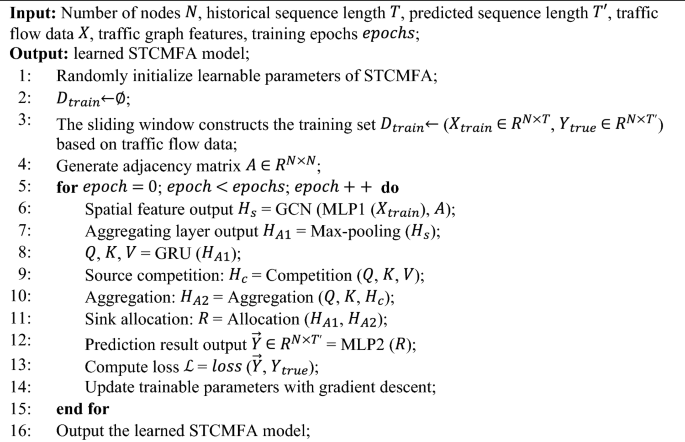
Training algorithm of STCMFA.


