
Conventional fossil fuels are the primary source of energy worldwide. However, they face the threat of depletion due to rapid consumption and the lengthy and costly process required to produce new fossil fuels1. Furthermore, it is the primary source of greenhouse gas emissions, such as carbon dioxide (CO₂), nitrous oxide (N₂O), and others. These emissions lead to climate changes, which threaten the environment and people’s lives2. Hence, finding new energy sources has become essential to combat climate change driven by traditional fossil fuels and to fulfill increasing energy needs as fossil fuel reserves dwindle3,4. Therefore, the countries have recently shifted toward renewable energy sources, such as wind, solar, and hydropower, which are derived from natural processes and have become essential alternatives due to their continuous generation, low costs, and significantly lower environmental impact. Among renewable energy sources, solar energy has attracted significant attention because of its reliability, low operating costs, and dependence on solar irradiance (SI)4. Accurate SI forecasting is increasingly crucial for managing solar energy systems effectively, since their power output depends on solar irradiance. The SI forecasting process is categorized into four groups based on forecast horizons: very short-term (critical for system monitoring), short-term (important for decision-making such as balancing demand and supply, committing units, and more), medium-term (used for planning maintenance schedules for power plants), and long-term (essential for site selection, solar plant installation, network operations, and related tasks)5.
Accurately predicting SI, especially in the short-term horizon, is essential for the stable and efficient operation of PV power plants. Therefore, in the literature, several SI forecasting models, divided into statistical models and machine learning (ML) and deep learning (DL) models, have been presented recently for handling this problem6. This study focuses on ML and DL models, as they are the most effective at capturing nonlinear dynamic relationships in SI data. Therefore, this section reviews recent studies on SI forecasting to highlight their strengths and weaknesses while identifying gaps that justify our study. Ahmed et al.6 introduced an ensemble SI forecasting model called PBNN, which combines three ML models—RF, XGB, and Categorical Boosting (CatBoost)—with a feedforward neural network (FFNN). The ML models serve as base learners trained on datasets, and their outputs are weighted by the FFNN to generate final predictions. Mutual information was used to select the best features, boosting the PBNN’s performance. The model was evaluated with two datasets—Islamabad and San Diego—and compared against several other models using various performance metrics, demonstrating its effectiveness. Results showed it outperformed all rivals, with improvements of approximately 47% and 74% for the respective datasets. However, it still risks getting stuck in local optima due to dependence on gradient-based optimizers for determining the optimal weights of the ML models.
This study7 presents a reliable DL framework for analyzing multi-scale variations in solar radiation. It combines feature engineering with transformation matrices, uses CNNs for local feature detection, and LSTMs for global uncertainty modeling. Trained on Tokyo meteorological data, the model shows high accuracy with an R² of 0.97 on unseen data. Zhu et al.8 presented a hybrid approach for predicting direct normal irradiance. This approach combined decomposition, clustering, the battle royale optimizer, and the CatBoost algorithm. Data from China’s Jiangsu province across all seasons were analyzed. Features were selected, decomposed via wavelet analysis, and grouped using sample entropy. The data were input into an optimized CatBoost model fine-tuned by the battle royale optimizer. This hybrid model could achieve outstanding results compared to several rival models. Díaz-Bedoya et al.9 explored SI forecasting with DL and ensemble models, using LSTM, RF, and ETs with meteorological data to improve accuracy. Zhang10 develops a hybrid forecasting model that combines sample entropy (SE) clustering, the CEEMDAN decomposition technique, support vector regression (SVR), and the grey wolf optimizer (GWO). Based on data from Jiangsu, China, the CEEMDAN-SE-GWO-SVR model outperforms the multi-layer perceptron (MLP) and the LSTM.
Naveed et al.11 introduced three innovative models for SI prediction: SEFMNN, Extreme Learning Machine (ELM), and XGB-Squared Error (XGB-SE). These models forecast shortwave SI in three Chinese regions—Guangdong, Shandong, and Zhejiang—and one in Saudi Arabia, Najran. SEFMNN integrates ANN, RF, and SVR to boost accuracy, while XGB-SE incorporates a specialized loss function for handling extreme data. All models aim to reduce overfitting and enhance efficiency and precision. Both XGB-SE and SEFMNN outperform ELM, significantly advancing SI forecasting for PV system planning. In12, various ML models, including linear regression, RF, decision trees, SVR, and gradient boosting, were tested for SI prediction. The simulation results demonstrate that RF is more effective, achieving an RMSE of 0.64 and surpassing linear regression by 19.47%. Mariappan13 introduced a hybrid DL model, CNN-SLSTM, to forecast daily global SI using measurement data and weather information. The recursive feature elimination technique based on RF was used to select the best subset of 14 key features. The hyperparameters of CNN-SLSTM were optimized using the slime mold algorithm. Through ten-fold cross-validation, the model was compared to several DL models, such as Gated Recurrent Unit (GRU), LSTM, CNN-LSTM, and various ML regressors like RF, SVR, and Decision Tree. The results indicate that CNN-SLSTM outperformed the other models.
Raju et al.14 introduced a hybrid DL model that combines LSTM networks with Chaotic Particle Swarm Optimization (CPSO). The DL model employs LSTM to identify complex temporal patterns in short-wave SI data. CPSO fine-tunes LSTM hyperparameters such as neurons, learning rate, batch size, dropout, and activation function to minimize prediction errors. The model’s performance is evaluated using metrics such as MAE, MAPE, RMSE, and the coefficient of determination. The best results are achieved for 60-minute-ahead forecasts during the rainy season. Li et al.15 introduced a Shadow-Attention Graph Neural Network (SAGNN) to predict SI for urban buildings. Alorf16 proposed an N-hours-ahead SI forecasting method that integrates variational mode decomposition (VMD) with an enhanced temporal fusion transformer (TFT). The approach employs VMD to decompose data into intrinsic mode functions (IMFs) and enhances TFT by incorporating a screening network and a GRU encoder–decoder. It can forecast at 1-hour intervals and other horizons. The experimental results demonstrate that this method outperforms several rival models.
Prajesh17 introduced the Light Gradient Boosting Machine (LightGBM), an ensemble learning method that reduces computation time and enhances forecasting accuracy. It employs a two-step process: using mutual information for feature selection, followed by an autoencoder for feature extraction to prevent overfitting. Additionally, the hyperparameters of LightGBM are tuned using the Honey Badger Algorithm to improve its performance on the SI forecasting problem. Testing on two datasets from the National Renewable Energy Laboratory demonstrates its advantages over benchmark models. In18, a novel GRU-TCN model that integrates a temporal convolutional network (TCN) and a GRU was proposed. It captures temporal features from SI data using the GRU and spatial features with the TCN. Both univariate and multivariate GRU-TCN models are used for ultra-short-term SI forecasting and are compared to several models, such as TCN, LSTM, and GRU. The empirical results show that the univariate model based on historical SI data is the best. Several other SI approaches have been recently presented for the SI forecasting, some of them are multivariate ML models19, convolution neural network-LSTM (CNN-LSTM)20, hybrid DL model21, EEMD–Transformer–GRU model22, SVR and Gaussian Process (GP) techniques23, Hybrid DL CNN-LSTM24, U-Shaped LSTM-Attention-Free Transformer (AFT)25, hybrid quantum neural network26, stacked ensemble learning-based correction model27, Quantum Neural Network28, a hybrid transformer-based framework29, ANN optimized by the Coati optimization algorithm30, and others31,32,33,34,35,36,37,38,39,40,41.
Although several studies have explored SI forecasting, they still struggle with modeling nonlinear data, require substantial computational costs, and often fail to select the optimal feature subsets to improve accuracy. Therefore, this study introduces a new multi-stage forecasting model called SIFA to accurately predict the SI, enhancing the stability and efficiency of PV power plants. The idea behind this model is based on employing a modern metaheuristic algorithm called the manta ray foraging optimizer (MRFO) to determine each base model’s contribution, which could lead to better predictive accuracy. We considered the metaheuristic algorithm due to its recent successful application in various ML tasks, achieving excellent results in a shorter time. Some of these tasks include student academic performance prediction42, anomaly detection in IoT networks43, ELM training tasks for medical datasets44, Power Quality Event Classification45, accurate diagnosis of Sjögren’s syndrome46, and feature selection tasks47,48,49,50. It is also worth noting that we chose the metaheuristic approach over the ANN employed in6, as the latter is more prone to falling into local optima and requires higher computational costs, as confirmed in our later experiments. Although several metaheuristic algorithms have been proposed, such as the Secant Optimization Algorithm51, Schrödinger optimizer52, and others53, we use MRFO in this study because it demonstrates stable and effective performance when handling various optimization problems in the literature.
The proposed SIFA approach consists of two stages: the feature selection stage using the RF-based sequential forward selection (SFS) method and optimized weight-based hybrid ML models. In the first stage, we use the SFS method to choose the optimal feature subset for improving SI predictions. This approach is integrated with the RF technique to evaluate various selected subsets, ultimately identifying the most effective one that leads to more accurate predictions. The number of estimators in the RF model as a hyperparameter affects the selection process. Tuning this hyperparameter is essential to improve the selected feature subset. Therefore, in this study, we present an enhanced version of the manta ray foraging optimizer (MRFO) that uses chaotic maps instead of traditional random generators to balance exploration and exploitation during optimization, called IWMRFO. This helps prevent stagnation in local optima and enhances convergence speed. This improved variant is used to tune the number of estimators in the RF model to achieve the optimal feature subset. The second stage involves using weight-based ML models to predict the SI based on the best feature subset. This stage combines three effective ML models—HR, ET, and XGB—based on a weight vector. This vector assigns a weight to each of the three models to determine their contribution to prediction accuracy. Estimating this weight vector is considered an optimization problem that must be solved accurately to determine each model’s contribution to improved predictive accuracy. Therefore, we employ the proposed IWMRFO to handle this problem. It is worth mentioning that ET, HR, and XGB are selected due to their effectiveness in modeling nonlinear features in the SI data. The proposed SIFA approach is evaluated using three popular datasets— the San Diego dataset, the Islamabad dataset, and the NASA SI dataset—and compared to several competing models based on various performance metrics: RMSE, MAE, MAPE, MSE, and R². SIFA, according to the experimental results, could significantly outperform all models across all performance metrics on the three datasets. The main contributions of this study are listed below:
a) Introducing A two-stage adaptive ensemble framework (SIFA) for accurate SI forecasting.
b) The first stage employs a wrapper-based feature selection method based on the RF-based SFS method to select the most informative features.
c) The second stage integrates three effective ML models HR, ET, and XGB using a weight vector to control the contribution of each base model in SIFA.
d) Tuning the number of estimators in the RF-based SFS method and the weight vector using an improved version of MRFO that employs chaotic maps instead of traditional random generators to balance exploration and exploitation during optimization.
e) Using three popular datasets San Diego, Islamabad, and NASA SI to evaluate the proposed approach, along with comparing it to several competing models based on various performance metrics: RMSE, MAE, MAPE, MSE, and R².
f) SIFA, based on the experimental results, was able to show lower error variability than all compared models on the three datasets, with improvements ranging from 10% to 95%.
This study is organized as follows: Sect. 2 introduces the enhanced MRFO, Sect. 3 explains the ET, XGB, and HR models, Sect. 4 outlines the proposed model, Sect. 5 details the experimental settings, Sect. 6 presents the results and discussion, and Sect. 7 presents conclusions and future research directions.
Enhanced manta ray foraging optimizer: WMQIMRFO
Recently, a new optimization algorithm called the MRFO, inspired by manta rays’ foraging behaviors chain, cyclone, and somersault—was developed for engineering optimization challenges54. In MRFO, the chain foraging behavior involves moving all individuals, except the first, towards both the individual in front of them and the best solution found so far. Meanwhile, the first individual is moved solely towards the best-so-far solution. This behavior is mathematically defined as follows:
$$\:\vec{x}_{i}^{{t + 1}} = \left\{ {\begin{array}{*{20}c} {\vec{x}_{i}^{t} + \vec{r} \cdot \:\left( {\vec{x}^{{\text{*}}} – \vec{x}_{i}^{t} } \right) + \alpha \cdot \:\left( {\vec{x}^{{\text{*}}} – \vec{x}_{i}^{t} } \right),\:\:\:\:\:\:\:\:\:\:\:\:\:\:\:\:\:if\:i = 1} \\ {\:\vec{x}_{i}^{t} + \vec{r} \cdot \:\left( {\vec{x}_{{i – 1}}^{t} – \vec{x}_{i}^{t} } \right) + \alpha \: \cdot \left( {\vec{x}^{{\text{*}}} – \vec{x}_{i}^{t} } \right),\:\:otherwise} \\ \end{array} } \right.$$
(1)
$$\:\alpha \: = 2 \cdot \:r\: \cdot \sqrt {\left| {{\text{log}}r} \right|}$$
(2)
where \(\:\overrightarrow{r}\) is a random vector in \(\:[0,\:1]\), \(\:{\overrightarrow{x}}^{*}\) stands for the best solution found so far, \(\:{\overrightarrow{x}}_{i}^{t+1}\) is the new solution, and \(\:{\overrightarrow{x}}_{i}^{t}\) is the current solution. The MRFO’s cyclone foraging mechanism consists of two parts. The first part emphasizes exploring areas near \(\:{\overrightarrow{x}}^{*}\) to accelerate convergence and is expressed as follows:
$$\:\vec{x}_{i}^{{t + 1}} = \left\{ {\begin{array}{*{20}c} {\vec{x}^{{\text{*}}} + \vec{r} \cdot \:\left( {\vec{x}^{{\text{*}}} – \vec{x}_{i}^{t} } \right) + \beta \: \cdot \:\left( {\vec{x}^{{\text{*}}} – \vec{x}_{i}^{t} } \right),\:\:\:\:\:\:\:\:\:\:\:\:\:\:\:\:\:if\:i = 1} \\ {\:\vec{x}^{{\text{*}}} + \vec{r} \cdot \:\left( {\vec{x}_{{i – 1}}^{t} – \vec{x}_{i}^{t} } \right) + \beta \: \cdot \:\left( {\vec{x}^{{\text{*}}} – \vec{x}_{i}^{t} } \right),\:\:otherwise} \\ \end{array} } \right.$$
(3)
$$\:\beta \: = 2 \cdot \:e^{{r_{1} \frac{{T_{{max}} – t + 1}}{{T_{{max}} }}}} \cdot {\text{sin}}\left( {2\pi \:r_{1} } \right)$$
(4)
where \(\:{r}_{1}\) represents a number randomly chosen in \(\:[0,\:1]\), \(\:t\) stands for the current iteration, and \(\:{T}_{max}\) stands for the maximum iteration. On the other hand, the second part emphasizes thoroughly exploring the search space to avoid getting stuck in local optima and improve the final results. This part is described as follows:
$$\:\vec{x}_{i}^{{t + 1}} = \left\{ {\begin{array}{*{20}c} {\vec{x}_{a}^{t} + \vec{r} \cdot \left( {\vec{x}_{a}^{t} – \vec{x}_{i}^{t} } \right) + \beta \: \cdot \:\left( {\vec{x}_{a}^{t} – \vec{x}_{i}^{t} } \right),\:\:\:\:\:\:\:\:\:\:\:\:\:\:\:\:\:if\:i = 1} \\ {\:\vec{x}_{a}^{t} + \vec{r} \cdot \:\left( {\vec{x}_{{i – 1}}^{t} – \vec{x}_{i}^{t} } \right) + \beta \: \cdot \:\left( {\vec{x}_{a}^{t} – \vec{x}_{i}^{t} } \right),\:\:otherwise} \\ \end{array} } \right.$$
(5)
$$\:{\overrightarrow{x}}_{a}^{t}=\overrightarrow{L}+\overrightarrow{r}\cdot\:\left(\overrightarrow{U}-\overrightarrow{L}\right)$$
(6)
where\(\:\:\overrightarrow{L}\) stands for the lower bound, and \(\:\overrightarrow{U}\:\)denotes the upper bound.
However, the second part was enhanced in55 by integrating it with the Morlet wavelet mutation (MWM) strategy to further strengthen the exploration operators and avoid stagnation in local optima. This strategy is used to update the current solutions based on a mutation probability (\(\:{p}_{m}\)). When this probability is smaller than a number randomly chosen in \(\:[0,\:1]\), the MWM strategy is implemented; otherwise, the traditional chain foraging equation defined in (5) is applied. The mathematical model of this strategy is as follows:
$$\vec{x}_{i}^{{t + 1}} = \left\{ {\begin{array}{*{20}c} {\vec{x}_{a}^{t} + \vec{r} \cdot \left( {\vec{x}_{a}^{t} – \vec{x}_{i}^{t} } \right) + \beta \cdot \left( {\vec{x}_{a}^{t} – \vec{x}_{i}^{t} } \right) + \sigma \cdot \left( {\vec{U} – \vec{x}_{i}^{t} } \right),~~~~~~~~~~~~~~~~~if~i = 1} \\ {\vec{x}_{a}^{t} + \vec{r} \cdot \left( {\vec{x}_{{i – 1}}^{t} – \vec{x}_{i}^{t} } \right) + \beta \cdot \left( {\vec{x}_{a}^{t} – \vec{x}_{i}^{t} } \right) + \sigma \cdot \left( {\vec{x}_{i}^{t} – \vec{L}} \right),~~otherwise} \\ \end{array} } \right.$$
(7)
$$\sigma = 1/\sqrt a \psi \left( {\varphi /a} \right)$$
(8)
$$a = s \cdot \left( {\frac{1}{s}} \right)^{{\left( {1 – \frac{t}{{T_{{max}} }}} \right)}}$$
(9)
where \(\:s\) is a constant value,\(\:\:\varphi\:\) is a number selected at random in the interval of \(\:-2.5a\) and \(\:2.5a\), and \(\:\psi\:\left(\varphi\:/a\right)\) represents the Morlet wavelet function:
$$\:\psi\:\left(x\right)={e}^{-{x}^{2}/2}\text{cos}\left(5x\right)$$
(10)
According to54, the preference for both parts during the optimization process depends on the current iteration, with the first part applied initially and the second part introduced as the optimization process advances. This implies that their preference is linearly weighted throughout the optimization, possibly leading to slow convergence in the early stages and stagnation in local optima later. To address this, the authors in55 adopted a nonlinear approach to enhance exploration and exploitation during different optimization phases. They employ sine, cosine, tangent, and logarithmic functions, defined as follows:
$$\:{C}_{f}=\text{sin}\left(\frac{\pi\:}{2}\cdot\:\frac{t}{{T}_{max}}\right)$$
(11)
$$\:{C}_{f}=1-\text{cos}\left(\frac{\pi\:}{2}\cdot\:\frac{t}{{T}_{max}}\right)$$
(12)
$$\:{C}_{f}=\text{tan}\left(\frac{\pi\:}{4}\cdot\:\frac{t}{{T}_{max}}\right)$$
(13)
$$\:{C}_{f}=\text{ln}\left(1+\left(e-1\right)\frac{t}{{T}_{max}}\right)$$
(14)
Finally, the tradeoff between both parts, according to one of the nonlinear approaches mentioned above, is defined as follows:
$$\:{\overrightarrow{x}}_{i}^{t+1}=\left\{\begin{array}{c}\left\{\begin{array}{c}\left(5\right),\:\:\:r<{p}_{m}\\\:\left(7\right),\:\:\:r\ge\:{p}_{m}\end{array}\right.\:\:\:\:\:\:\:\:\:\:\:\:\:\:\:\:\:\:\:\:\:\:\:\:\:if\:{r}_{1}>{C}_{f}\\\:\left(3\right),\:\:\:\:\:\:\:\:\:\:\:\:\:\:\:\:\:\:\:\:\:\:\:\:otherwise\end{array}\right.\:$$
(15)
where \(\:r\) and \(\:{r}_{1}\) are numbers randomly chosen in \(\:[0,\:1]\). Finally, the somersault foraging mechanism consistently updates the individual based on the best solution identified so far, enhancing exploitation and speeding up convergence to the global optimum. This mechanism is defined by:
$$\:\vec{x}_{i}^{{t + 1}} = \:\vec{x}_{i}^{t} + S \cdot \:\left( {r_{2} \cdot \:\vec{x}^{{\text{*}}} – r_{3} \cdot \:\vec{x}_{i}^{t} } \right)$$
(16)
where \(\:S\) represents the somersault factor and is advised to be configured at 2, and \(\:{r}_{2}\) and \(\:{r}_{3}\) represent numbers randomly chosen in \(\:[0,\:1]\). To further enhance the exploitation operator of the MRFO algorithm, a quadratic interpolation (QI) strategy is integrated into the updated population, as described in55, to accelerate convergence and improve accuracy. Finally, integrating the QI, MWM, and nonlinearity mechanisms with the standard MRFO could produce a more effective variant, called WMQIMRFO (referred to as WMRFO for short), featuring stronger exploration and exploitation operators in the optimization process to improve convergence speed and prevent stagnation in local optima.
Machine learning models: Overview
This section reviews the core ML models employed in developing the proposed model, including HR, XGB, and ET regression.
Huber regression model
In 1964, Peter J. Huber introduced the Huber Regressor (HR) to address the important issue of sensitivity in linear regression. HR combines the advantages of linear and robust regression for reducing the influence of outliers on the model’s accuracy. It uses the Huber loss function, which acts quadratically for small residuals—similar to ordinary least squares—and linearly for large residuals, like robust regression, ensuring efficiency while reducing sensitivity to outliers56. The Huber loss function is defined by
$$\:H\left({r}_{i}\right)=\left\{\begin{array}{c}\frac{1}{2}{r}_{i}^{2}\:\:\:\:\:\:\:\:\:\:\:\:\:\:\:\:\:\:\:\:\:\:\:\:if\:\left|{r}_{i}\right|\le\:\eta\:\\\:\eta\:\left(\:\left|{r}_{i}\right|-\frac{1}{2}\:\eta\:\right)\:\:\:Otherwise\end{array}\right.$$
(17)
where \(\:{r}_{i}\) represents the difference between the predicted and estimated values for the ith sample, and \(\:\eta\:\) is a threshold parameter that defines the point at which the loss function switches from quadratic to linear. The HR model involves hyperparameters like \(\:\eta\:\) in (17), max_iter for weight updates, and alpha for regularization to prevent overfitting. Accurate estimation of these hyperparameters is crucial for improving HR’s prediction for SI.
Extra trees regression
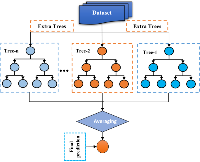
The ET regression model is an ensemble learning method similar to RF, applicable for both classification and regression57. As shown in Fig. 1, ET consists of several decision trees (DTs). Unlike RF, where each tree is trained on a bootstrap sample, ET builds all trees using the entire training dataset. ET adds stochasticity by randomly choosing split thresholds for each feature, which improves generalization and reduces overfitting. The final prediction results from averaging the outputs of all DTs, as detailed in the following equation57:
$$\:{F}_{p}=\frac{1}{n}\sum\:_{i=1}^{n}{T}_{i}\left(\overrightarrow{x}\right)$$
(18)

ET regression’s architecture.
where \(\:{F}_{p}\) denotes the final forecast for the input sample (\(\:\overrightarrow{x}\)), \(\:n\) is the number of decision trees in the ensemble, and \(\:{T}_{i}\) represents the output of the \(\:ith\) decision tree for \(\:\overrightarrow{x}\).
Extreme gradient boosting
Boosting algorithms combine weak classifiers to create a strong learner that improves data interpretation and increases prediction or classification accuracy58. There are several boosting algorithms found in the literature, such as Adaboost59, histogram-based gradient boosting (HGB), gradient boosting60, CatBoost61, and XGB. The XGB algorithm is an optimized and scalable gradient boosting method aimed at achieving high predictive accuracy and efficiency62,63. It constructs an ensemble of weak learners typically decision trees by adding each one sequentially, with each new tree focusing on correcting the residual errors from previous trees. The model utilizes a regularized loss function that combines a differentiable error metric with a regularization term, which helps limit the model’s complexity. This approach reduces the risk of overfitting and improves the model’s ability to generalize. XGB includes several algorithmic improvements, such as second-order gradient optimization, shrinkage (learning rate), and parallelized tree building. These enhancements increase its accuracy and speed. As a result, XGB has become a leading ensemble method for both classification and regression tasks, particularly in large-scale and high-dimensional datasets. The final model prediction is computed by summing the outputs of all trees, as defined in the following formula:
$$\:{F}_{p}^{k}=\sum\:_{i=1}^{n}{T}_{i}\left(\overrightarrow{{x}_{k}}\right)$$
(19)
where \(\:{F}_{p}^{k}\) stands for the predicted value for the \(\:kth\) sample, and \(\:{T}_{i}\) represents the forecasting of the \(\:ith\) tree for the \(\:kth\) sample.
Proposed model: SI forecasting approach (SIFA)
This section explains the proposed methodology, which combines three effective ML models whose weights are optimized by the enhanced WMRFO. These optimized weights determine each model’s contribution to the final predictions, enabling the selection of a combination with strong generalization ability and high predictive accuracy. Additionally, in the preprocessing step, we use the RF-based sequential forward selection (SFS) technique to choose the optimal subset of features, thereby improving the model’s performance. The number of estimators in the RF—a hyperparameter affecting the model’s performance—is optimized using the proposed IWMRFO. Overall, the proposed model involves feature selection with RF-based SFS, IWMRFO enhanced with chaotic maps, and a weighted hybrid ML. These steps are explained in detail in the following subsections.
RF-based SFS technique: The feature selection step
The feature selection step is crucial for several ML tasks because of its role in improving classification accuracy and reducing computational costs. This step is performed using various techniques divided into three classes: wrapper-based, filter-based, and embedded-based. Filter-based techniques use statistical metrics to assess the correlation between each independent feature and the target variable. These methods rely on measures like correlation coefficients, mutual information, chi-square statistics, or ANOVA F-values to gauge the strength of the association; therefore, they are known as model-independent methods. Features that exhibit little or no correlation with the target are deemed irrelevant and are removed from the dataset. The wrapper-based method is dependent on the model, as it utilizes an ML model to evaluate the quality of the selected feature subset. The RF-based SFS method falls into this category, starting by evaluating each feature individually with RF and storing the one with the lowest MSE in a feature subset array. In the next iteration, the remaining features are tested one by one in combination with those already in the array, and any feature that improves performance is added to the array. This iterative process repeats until the number of required features is selected. Finally, the resulting subset comprises the most informative, non-redundant features identified by the RF model. However, the RF model has some hyperparameters that influence the quality of the selected features; the most important one is the number of estimators (decision trees). This hyperparameter needs to be estimated accurately to help select the best feature subset with the aim of improving predictive accuracy and reducing computational costs. Therefore, in this study, we use the proposed IWMRFO discussed in the next section to determine the optimal value for this parameter. Finally, the pseudocode for the RF-based SFS technique is provided in Algorithm 1. This algorithm aims to achieve high effectiveness in reducing dimensionality, eliminating redundancy, and enhancing model efficiency without compromising predictive accuracy.
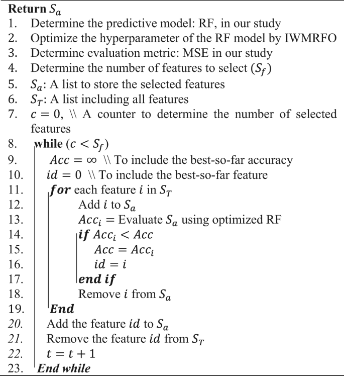
Pseudocode of RF-based SFS.
Proposed chaotic-based WMRFO: IWMRFO
Chaotic maps can replace the WMRFO algorithm’s traditional pseudorandom numbers by generating a sequence of values using a deterministic recursive equation that begins with a randomly initialized seed value, improving the algorithm’s exploration ability and convergence stability. Chaotic sequences are deterministically random, exhibiting characteristics such as ergodicity and sensitivity to initial conditions, which help diversify the search process, thoroughly explore the search space, and reduce the risk of premature convergence to local optima. Additionally, the deterministic nature of chaos helps maintain stability during optimization. By substituting random distributions with chaotic sequences, WMRFO can better balance exploration and exploitation, resulting in improved convergence accuracy and higher-quality solutions. This study employs ten one-dimensional maps, commonly used in various literature sources24,25, to generate chaotic sets. Given their diverse behaviors, we compare the effectiveness of the proposed MWRFO algorithm with several of these chaotic maps to identify which yields the most accurate results. The mathematical definitions for these 10 chaotic maps are summarized in Table 164,65. These maps are designed to replace some random numbers—not all—in WMRFO equations to encourage diversity in the algorithm’s search behaviors and achieve higher-quality solutions. The first is the random number in (15), which controls the balance between the two parts of the cyclone foraging mechanism. When chaotic maps are used, this equation is redefined as follows:
$$\:{\overrightarrow{x}}_{i}^{t+1}=\left\{\begin{array}{c}\left\{\begin{array}{c}\left(5\right),\:\:\:r<{p}_{m}\\\:\left(21\right),\:\:\:r\ge\:{p}_{m}\end{array}\right.\:\:\:\:\:\:\:\:\:\:\:\:\:\:\:\:\:\:\:\:\:\:\:\:\:if\:{C}_{i}>{C}_{f}\\\:\left(3\right),\:\:\:\:\:\:\:\:\:\:\:\:\:\:\:\:\:\:\:\:\:\:\:\:otherwise\end{array}\right.\:$$
(20)
where \(\:{C}_{i}\) denotes a number generated by one of the ten chaotic maps. This update adjusts the balance between the exploration operators in (5–6) and the exploitation operators in (3), helping to prevent local optima traps and accelerating convergence.
In addition, the random vector in (7) is also replaced by the chaotic maps to improve the exploration operator along the optimization process. However, this equation will strongly motivate exploration operators, which can increase population diversity but slow down convergence. To address this, this equation is modified to dynamically steer the search: it emphasizes exploitation near \(\:{\overrightarrow{x}}^{*}\) when the chaotic value is below 0.5 and encourages exploration around \(\:{\overrightarrow{x}}_{a}^{t}\) when it exceeds 0.5. As the chaotic value nears 0.5, the method gradually balances exploration and exploitation. (7) after modification is defined as follows:
$$\:\vec{x}_{i}^{{t + 1}} = \left\{ {\begin{array}{*{20}c} {\overrightarrow {{x_{{Ba}} }} + \overrightarrow {{C_{3} }} \cdot \:\left( {\vec{x}_{a}^{t} – \vec{x}_{i}^{t} } \right) + \beta \: \cdot \:\left( {\vec{x}_{a}^{t} – \vec{x}_{i}^{t} } \right) + \sigma \: \cdot \:\left( {\vec{U} – \vec{x}_{i}^{t} } \right),\:\:\:\:\:\:\:\:\:\:\:\:\:\:\:\:\:if\:i = 1} \\ {\:\overrightarrow {{x_{{Ba}} }} + \overrightarrow {{C_{3} }} \cdot \:\left( {\vec{x}_{{i – 1}}^{t} – \vec{x}_{i}^{t} } \right) + \beta \: \cdot \:\left( {\vec{x}_{a}^{t} – \vec{x}_{i}^{t} } \right) + \sigma \: \cdot \:\left( {\vec{x}_{i}^{t} – \vec{L}} \right),\:\:otherwise} \\ \end{array} } \right.$$
(21)
$$\:\overrightarrow{{x}_{Ba}}={C}_{2}\text{*}{\overrightarrow{x}}^{\text{*}}+\left(1-{C}_{2}\right)\text{*}{\overrightarrow{x}}_{a}^{t}$$
(22)
where \(\:\overrightarrow{{C}_{3}}\) denotes vector generated by one of the ten chaotic maps, and \(\:{C}_{2}\) denotes a number generated by one of the ten chaotic maps. The pseudocode for the enhanced WMRFO (IWMRFO) is outlined in Algorithm 2. It starts by creating an \(\:N\:\times\:\:D\) matrix, where \(\:N\) is the population size and \(\:D\) is the problem’s dimension. This matrix is initialized randomly within the problem’s lower and upper bounds. All solutions in the matrix are then evaluated individually, and their fitness scores are compared. The solution with the highest accuracy is selected as the best so far. The population is subsequently refined using IWMRFO’s update schemes and re-evaluated to improve \(\:{\overrightarrow{x}}^{*}\), as detailed in Lines 6–28. This cycle repeats until the maximum number of function evaluations is reached, as indicated in Line 7. Upon completing the optimization process, the final best-so-far solution is returned.
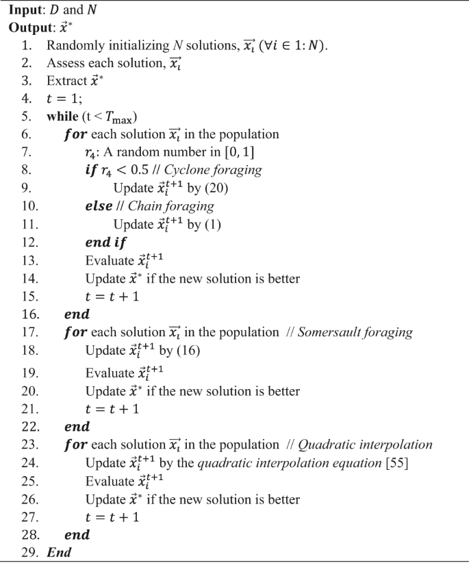
Optimized weight-based hybrid ML: SIFA
This study introduces a weight-based hybrid ML model (SIFA) that combines three robust algorithms: ET, HR, and XGB. These models are integrated using a weight vector that assigns each model’s contribution to the final prediction accuracy. Optimizing these weights is crucial for improving the model’s generalization capability. To achieve this, the proposed IWMRFO is employed to identify the most effective weights, thereby increasing the accuracy of SI predictions. Essentially, this approach can be formulated as a mathematical equation composed of variables and coefficients: coefficients stand for the fixed predictions of each base model, and the variables represent the weights optimized by the proposed algorithm. The following equation describes the mathematical model of our approach:
$$\:\overrightarrow{{P}_{F}}={w}_{1}{\overrightarrow{x}}_{1}+{w}_{2}{\overrightarrow{x}}_{2}+{w}_{3}{\overrightarrow{x}}_{3}$$
(23)
where \(\:{w}_{1}\), \(\:{w}_{2}\), and \(\:{w}_{3}\) represent the weights assigned to the predictions of the ET, HR, and XGB models, respectively, and \(\:{\overrightarrow{x}}_{1}\), \(\:{\overrightarrow{x}}_{2}\), and \(\:{\overrightarrow{x}}_{3}\) denote the forecasts/coefficients produced by these models.
This equation can include more than three models if it improves prediction accuracy. We rely on these three models because, after extensive testing, we found they are the most effective for better SI predictions. The variables, or weights, in this equation are optimized using the proposed IWMRFO algorithm. Initially, the SI dataset undergoes preprocessing and is split into 80% training data and the remaining samples for testing. Each base ML model is then trained independently. Afterward, IWMRFO explores the search space to find the best combination of these models, aiming to improve overall generalization.
The flowchart of the proposed SIFA framework is shown in Fig. 2. In this figure, the input SI dataset is initially preprocessed using normalization to improve learning. Afterward, feature selection is performed to identify the most informative features, which could improve prediction accuracy. The dataset is then split into training and testing sets, with the training data used to train the three main ML models: HR, XGB, and ET. The trained models are then input to the IWMRFO, which begins its optimization process by creating an \(\:N\:\times\:\:D\) matrix. Each solution in this matrix is randomly initialized within the lower and upper bounds of the various ML components, as described in the experiments section. These solutions are then substituted into (23) to produce predicted values for the dataset samples. These predictions are evaluated by comparing them to the actual values using the MSE objective function defined below:
$$\:MSE=\frac{1}{n}\sum\:_{i=1}^{n}{({Y}_{i}-\stackrel{\sim}{{Y}_{i}})}^{2}$$
(24)

Flowchart of the proposed SIFA model.
where \(\:n\) stands for the number of samples, \(\:{Y}_{i}\) is the estimated value for the \(\:\text{i}\text{t}\text{h}\) sample, and \(\:\stackrel{\sim}{{Y}_{i}}\) represents the actual value for this sample.
The MSE values of different solutions within the population are compared, and the solution with the lowest MSE is identified as the best-so-far. This solution subsequently guides the optimization process to improve the quality of the remaining solutions. IWMRFO begins by iteratively updating candidate solutions within the population to generate new ones. Each new solution is substituted into (23) to produce predictions for the dataset samples. These predictions are then evaluated using the MSE objective function to determine each candidate solution’s fitness value. The fitness values are used to update the best-so-far solution whenever a better candidate is found. The IWMRFO optimization continues until \(\:{T}_{\text{m}\text{a}\text{x}}\) is reached. After completing the process, the best-so-far solution is returned and substituted into (23). This equation is then used to test the model’s ability to generalize. Each base model makes predictions on the testing dataset, which are assigned to their respective variables in (23) to produce the final predictions. These predictions are evaluated using multiple performance metrics, such as RMSE, MSE, R², and others discussed later.


