Optimizing support vector machine (SVM) by social spider optimization (SSO) for edge detection in colored images

The proposed method for edge detection in color images is performed at two levels. At the first level, image edges are approximated through a SVM optimized by the SSO algorithm using the grayscale image. Then, at the second level, the SSO algorithm is used to improve the approximated edges based on the comparison with pairwise combinations of color layers in the original image. It should be noted that the proposed method assumes that the input image is presented in RGB color system. Based on this, the steps of the proposed method for edge detection in color images are as follows:

1. 1.

   Edge approximation based on SVM and SSO.

2. 2.

   Edge improvement based on SSO and the difference with color layer combinations.

The architecture of the proposed method is illustrated in Fig. 1 as a diagram. In this figure, the steps related to each phase of training (SVM model optimization) and testing (edge detection in new images) are separated from each other.

The proposed method begins with optimizing the SVM model based on the training samples of the database using the SSO algorithm. For this purpose, the RGB training images are first converted to the grayscale color system, and then these samples, along with their ground-truth edges, are used as the input training data for the SVM model. The proposed SVM model utilizes a RBF kernel function, and its parameters are optimized using the SSO algorithm. The goal of this process is to achieve an SVM model with the least error in approximating the edges of the grayscale image. The result of this process is an SVM model with the best discovered configuration by the SSO algorithm, which is used for the initial approximation of edges in test images. The approximated edges identified through this model are compared with pairwise combinations of color layers, and an effort is made to minimize the difference between the edge pixels and the identified boundaries in different layer combinations using the SSO algorithm. The outcome of this process is the detected edges in the image.

Edge approximation based on SVM and SSO

The proposed method starts with the initial approximation of image edges using the combination of SVM and SSO. For this purpose, a training set of RGB images is used, where for each RGB image, there is a binary matrix indicating the background edges of the image. This training set is used as the training samples for the SVM model. At the beginning of this stage, each RGB image is first converted to the grayscale color system. Then, the training records are formed based on the pixel values present in the grayscale image. To do so, the intensity information of the current pixel and the intensity of pixels within the neighboring radius R are extracted. By transforming these values into a vector form, a training record for the SVM model is constructed. Additionally, the corresponding value for each pixel in the ground-truth edge image is considered as the target label for that training sample. Figure 2 illustrates the process of forming a training record for a sample pixel. In this figure, the assumed pixel is represented as x. Assuming R = 1, the length of the feature vector will be 9, and if R = 2, then the features of each pixel will be described in a vector form with a length of 25. It should be noted that, considering the learning properties of the SVM model, the order of features does not affect the final result. Also, for pixels on the image boundary that fall outside the image extent, the values of their missing neighboring pixels are set to zero during training data generation.

After forming the training records based on the training RGB images and their ground-truth edges, the SVM model is trained and optimized. The proposed method utilizes an SVM model with a RBF kernel as an initial estimator for the image edges. SVM, a well-known binary classifier, has been widely used in various problem-solving scenarios. This classifier attempts to create a boundary that separates the samples of the two target classes. By creating this boundary, the samples of each class will reside in a region known as the hyperplane. The margin, which represents the minimum distance between the samples and the boundary between the hyperplanes, is considered. The objective of the SVM training algorithm is to maximize the margin between the hyperplanes²⁵.

Since the relationship between the input variables (pixel intensity and its neighbors) and the target classes (pixel membership in an edge) in the discussed problem is nonlinear, a non-linear kernel function called the RBF has been used to solve this problem with SVM. The radial basis function kernel is formulated as follows in the SVM model²⁶:

In the above relationship, \({x}_{i}.{x}_{j}\) represents the dot product of the feature vectors for samples \({x}_{i}\) and \({x}_{j}\). This is a common kernel trick used in SVMs with RBF kernels. Moreover, γ represents the coefficient of the kernel function. On the other hand, the number of samples belonging to the two classes, positive (edge members) and negative (background members), is unbalanced. This imbalance can lead to a decrease in training quality and an increase in errors. To address this issue in the SVM model, a correction parameter is adjusted separately for each class. In this case, the optimization problem of the SVM model can be described as follows²⁶:

In the above relationship, w represents the normal vector of the hyperplane, and b determines the margin coefficient. Additionally, \({x}_{i}\) represents the i-th training sample, and \({d}_{i}\) describes the corresponding label for that sample. Moreover, \({\xi }_{i}\) represents the slack variable. For a sample i which has been correctly classified \({\xi }_{i}=0\) and otherwise, \({\xi }_{i}\) is the distance between i and its hyperplane. Finally, \({C}_{+}\) and \({C}_{-}\) are the correction parameters for the positive and negative classes, respectively.

For problems with balanced number of samples in target classes, the correction parameters for the positive and negative classes can be considered the same. But, the edge detection task is a highly imbalanced problem that the number of samples of the positive category (edge pixels) is insignificant compared to the number of samples of the negative category (background pixels). For this reason, the correct performance of the SVM model depends on the precise setting of the correction parameters for the positive and negative classes. Accordingly, an SVM model can be optimized using the correction parameters \({C}_{+}\) and \({C}_{-}\), as well as the radial basis coefficient γ. This process can be formulated as an optimization problem that utilizes the SSO algorithm in the proposed method.

Next, the defined structure for each solution vector and the evaluation procedure for objective function will be presented. Then, the optimization steps of the SVM model based on the SSO will be described.

As mentioned, in the process of configuring the SVM model using SSO, the goal is to determine the optimal values for the parameters \({C}_{+}\),\({C}_{-}\), and γ. Each of these parameters is considered as an optimization variable that can take real values. Therefore, the length of each solution vector will be 3. The search bounds of each optimization variable has been determined experimentally. In each solution vector, the search bounds for \({C}_{+}\) and \({C}_{-}\) are set as \(\left[{10}^{-2},3.6\times {10}^{4}\right]\). This bound, covers all possible valid combinations of hyperparameters \({C}_{+}\) and \({C}_{-}\) in edge detection problem. On the other hand, the search bounds for the γ parameter are set as \(\left[{10}^{-10},{10}^{2}\right].\)

Defining the objective function can be considered as the key component in solving optimization problems. Because based on the objective function, the quality of a solution can be determined. In the proposed method, the objective function is defined based on a validation error criterion. Thus, to evaluate the objective value of each solution vector (the optimality of values specified for SVM hyperparameters), first, the considered values for hyperparameters \({C}_{+}\),\({C}_{-}\), and γ are extracted from the solution vector and these values are applied to the SVM model. This, will result in a configured SVM model based on the parameters specified in that solution vector. Then, the configured SVM model is trained on the training data. Finally, by applying the validation samples to the trained model, the training error is considered as the objective function.

In the above equation, E represents the number of misclassified records in the validation set. In other words, it signifies the number of validation samples for which the SVM model, configured with the parameters from a specific solution vector, produced an output class different from the actual class label. Additionally, the parameter N represents the total number of records in the validation set.

Minimizing this objective function value is the goal of the SSO algorithm. A lower value indicates better performance of the SVM model on unseen data (validation set) and translates to a more accurate edge detection outcome. The basic idea of SSO algorithm is using the cooperative behavior of social spiders in colony. This algorithm works based on search agents that are modeled as spiders. Unlike most swarm intelligence methods where search agents have the same behavior; In SSO, two types of search agents (male and female spiders) with different behavior are defined, which can lead to a more efficient approach of searching the problem space. The SSO algorithm starts by initializing the population. Then an iterative mechanism is used for finding the optimal solution. At the beginning of each search cycle, the objective value of each spider is calculated. Then, based on the calculated weight, a weight value is assigned to each spider which can model the attractiveness of the spider for others²⁷:

In the above equation, the term \(fitnes{s}_{i}\) represents the calculated objective value for solution i, while “worst” and “best” indicate the worst and best objective values in the current population, respectively. The weight of each spider is used to calculate the vibration level of each spider as follows²⁷:

In the above equation, \({w}_{j}\) represents the weight assigned to spider \(j\) according to Eq. (4), and \(d\) represents the distance between two spiders. It should be noted that each spider, like \(i\), accepts only three types of vibrations. The first type is represented as \(n\) and indicates vibrations generated by a closer spider with a higher weight. The second type represents vibrations generated by a female spider and is only accepted by male spiders. Finally, the third type represents vibrations generated by the best spider in the population. In the next step of SSO cycles, the position of each spider is updated. SSO uses two different strategies for simulating the movement pattern of male and female spiders. The position of female spiders is updated based on their current position and received vibrations as follows²⁷:

In the above equation, the parameters \(\alpha\), \(\beta\), and \(\delta\) are random numbers in the range [0, 1]. Also, \({s}_{n}\) and \({s}_{b}\) represent the position of the neighboring and the best spider, respectively. Finally, \({f}_{i}(k)\) represents the current position of spider i, and \({f}_{i}\left(k+1\right)\) describes its new position. On the other hand, the position of male spiders is updated by considering the vibration from female spiders, also²⁷:

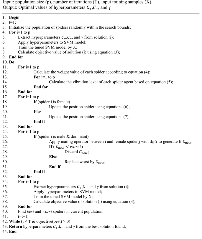
In the above equation, \({s}_{f}\) represents the position of the nearest female spider. At the final step of each cycle in SSO, the mating and survival operators are applied to the population. If a male spider is dominant, it can perform a mating operation with female spider within range r. This will result in a new solution such as \({C}_{new}\). In order to simulate the survival operation for \({C}_{new}\), its objective value is compared with worst. If \({C}_{new}<worst\), then the new solution is replaced with the worst solution in the population; otherwise, \({C}_{new}\) is discarded. The described cycle is repeated for a predetermined number of times. In the following, the pseudo code of proposed procedure for SVM optimization by SSO algorithm is presented.

After executing the above steps, the determined configuration in the solution vector with the minimum objective value is applied to the SVM model, and this model is used for the initial estimation of edges in the test samples. To do this, the test image is first converted to a grayscale system, and then the feature vectors of each pixel in the image are formed based on the process described at the beginning of this section. By feeding these vectors to the optimized SVM model, the membership of each pixel in the image to the edge region is determined. The binary matrix resulting from the aggregation of the SVM model outputs is considered as the initial approximation of the edge map of the grayscale image.

Edge enhancement based on SSO and difference with color channels combinations

After creating the edge approximation matrix, the SSO algorithm is used to improve the edge regions in the image. The search steps for finding the optimal solution by the SSO algorithm in this step are similar to the previous step, with the difference that a different structure is used for encoding the solution vector and evaluating its objective value. This structure is explained through an example. Consider an edge approximation matrix (result of the previous step) as shown in Fig. 3a. The SSO algorithm in this step attempts to match each pixel on the edge with the intensity values of the three matrices L₁, L₂, and L₃ by displacing them. In this case, each edge pixel is considered as an optimization variable that can be moved by at most one pixel in the solution vector. In Fig. 3a, each edge pixel is represented by optimization variables v₁ to v₈. Thus, for this sample image, the length of the solution vector will be 8. An example solution vector for this example is shown in Fig. 3b. Each element of this vector corresponds to one of the optimization variables (edge pixels v₁ to v₈), and the value in each position of the solution vector determines the displacement of that edge pixel. The encoding scheme for the solution vector for each pixel is shown in Fig. 3d. According to this figure, the number 0 indicates no displacement of the edge pixel, and numbers 1 to 8 indicate displacement in one of the surrounding directions with a radius of 1. By applying the solution vector shown in Fig. 3b to the edge matrix in Fig. 3a, the resulting image will be as shown in Fig. 3c, where pixels v₁, v₂, v₆, and v₈ are displaced according to the assumed solution vector pattern.

With these explanations, each solution vector of the SSO algorithm in the second step of the proposed method will have a length equal to the number of pixels located on the edge in the initial approximation image. This length indicates the number of optimization variables, and each optimization variable is described by an integer in the range [0, 8].

After editing the edges based on the solution vector, the fitness evaluation is performed by comparing the values of edge pixels in pairwise combinations of color layers in the original image. For this purpose, each pairwise combination of color layers, in the form of <RG, GB, BR> , is transformed into a matrix using the following equation:

In the above equation \({I}_{1},{I}_{2}\) represent two different layers of the RGB image, and Lc represents the uniform combination of these two layers. By applying the above equation to the combinations of <RG, GB, BR> layers, three matrices, denoted as L₁, L₂, and L₃, will be obtained, corresponding to the combination of RG, GB, and BR layers, respectively. In this case, the fitness evaluation of the solution vector S is performed using the following equation:

In the above equation, \({L}_{i}^{j}\) represents the edge pixel value in the layer \({L}_{i},(i=\mathrm{1,2},3)\) and \(N\left({L}_{i}^{j}\right)\) denotes the sum of values of its neighboring pixels (within a radius of 1). Additionally, the standard deviation function is shown as \(std\left(.\right)\). Finally, |S| represents the number of optimization variables or the number of edge pixels. According to the equation, to evaluate the fitness of each solution vector, the edge pixels are first moved according to the displacement vector, and then the mean standard deviation at the positions corresponding to the edge pixels in the combined layer combinations L₁, L₂, and L₃ is calculated. By performing this process, we can ensure that the edge pixels are located on the borders of the regions in the color layers of the initial image, and the maximum distinction between the color regions can be achieved based on the edges. Since the goal of the optimization algorithm is to maximize the mean standard deviation, Eq. (9) is formulated in an inverse form, and the addition of 1 is included to prevent division by zero (for completely uniform regions in the images). With these explanations, the SSO algorithm in the second step of the proposed method attempts to edit the positions of the edge pixels in the initial approximation in a way that minimizes Eq. (9). The pattern obtained from the optimal solution vector in this step will be applied to the edge approximation matrix to obtain the output of the proposed method based on it.