This section outlines the comprehensive experimental framework employed to develop and evaluate optimized image preprocessing strategies for neural network-based defect detection in industrial automation. The approach integrates systematic data acquisition, distinct preprocessing paradigms, genetic algorithm optimization, convolutional neural network architecture, and rigorous statistical evaluation methodologies35,36.
The experimental design follows established principles for computer vision research, incorporating stratified sampling, controlled variables, and statistical frameworks for model evaluation. Our methodology adopts a design science approach that operates at the interface of creative design and explanatory science to create and test innovative preprocessing optimization solutions. The experimental framework consists of stratification, sampling, and estimation components that allow efficient model evaluation while maintaining statistical rigor.
Dataset acquisition and partitioning
In data acquisition, images of all required products are captured using a Basler sensor and a Baumer camera under varying lighting conditions and stored according to the respective product categories. For the use case presented in this article, the dataset is organized into three product categories, each divided into two classes: Defective (D) and Non-Defective (ND), as shown in Table 1.
Dataset partitioning follows stratified sampling methodologies to ensure proportional representation across all stratification criteria while maintaining the statistical rigor necessary for unbiased model training and evaluation. The experimental dataset comprises 543 images (297 defective, 246 non-defective) distributed across three industrial products: Product 1 (111 defective, 94 non-defective), Product 2 (65 defective, 80 non-defective), and Product 3 (121 defective, 72 non-defective). For Product 1, the defective class includes multiple visually distinct defect types (e.g., surface scratches, local contamination, and shape irregularities), whereas Product 2 exhibits fewer but more homogeneous defect patterns. In contrast, Product 3 primarily contains a single dominant defect type with relatively consistent appearance across samples. Lighting conditions also differ across products: images for Products 1 and 2 were captured in a laboratory setup with fixed but moderately controlled illumination, while Product 3 was acquired directly on an industrial production line using a dedicated machine-vision lighting arrangement with highly uniform illumination. Each product therefore exhibits a moderate but realistic class imbalance, and stratified partitioning was applied to preserve the original defective/non-defective ratios in both training and test subsets. A stratified 80/20 training-to-test split was consistently applied in all experimental settings, resulting in approximately 434 training images and 109 test images throughout the full dataset.
To evaluate how the size of the training set influences model performance, the number of training images was systematically varied by randomly selecting n images per product class, where n corresponds to predetermined sample sizes (8, 12, 16, 20, 24, 28, and 32 images for different products) while maintaining the stratified split ratio throughout each experiment. This approach enables the identification of the minimum effective sample size required for each preprocessing condition and product category.
Image preprocessing methodologies
The investigation employs three distinct preprocessing paradigms that enable a comprehensive comparative analysis of automated versus manual optimization approaches, providing empirical evidence for the effectiveness of the evolutionary algorithm in industrial computer vision applications. As shown in Table 1, each product can be classified into two classes–Defective (D) and Non-Defective (ND)–with the images serving as representative samples for each class.
Baseline methodology: raw image processing
As illustrated in Fig. 2, the baseline condition uses unprocessed images as direct CNN input, establishing fundamental performance benchmarks against which preprocessing interventions are evaluated. Raw image processing maintains original pixel intensities, spatial dimensions, and color characteristics as acquired from imaging systems, ensuring that baseline results do not suffer artificial enhancement bias. Essential normalization operations include scaling the value of the pixels in a range and standardized resizing to uniform dimensions using bilinear interpolation while preserving aspect ratios.

Manual preprocessing optimization
As illustrated in Fig. 3, traditional preprocessing is based on systematic expert-driven parameter selection informed by domain knowledge and established industrial computer vision practices. The manual optimization process involves designing comprehensive preprocessing pipelines, where computer vision specialists iteratively evaluate and refine filter combinations through trial-and-error to identify the most effective configuration for each product category.

Workflow for image preprocessing.
Comprehensive Filter Library Manual preprocessing utilizes a comprehensive library of 48 distinct preprocessing operations shown in Table 2, including binarization with threshold optimization, morphological operations (dilation, erosion, opening, closing), edge detection methods (Sobel, Canny, Roberts, Prewitt, DoG, Laplacian), filtering techniques (Gaussian, median, bilateral, low-pass, high-pass), geometric transformations (scaling, rotation, translation), and advanced techniques (watershed segmentation, wavelet transforms, active contours).
Parameter Optimization Process Each preprocessing operation requires careful parameter tuning based on the characteristics of each product category. For example, binarization thresholds are selected using histogram-based intensity distributions (typical ranges: 80–140). Morphological operations employ kernel sizes between 3\(\times\)3 and 11\(\times\)11 pixels, chosen according to the shape and scale of the defect, while the edge detection parameters are adjusted based on local edge-strength statistics.
Sequence design methodology Manual preprocessing pipelines are designed for each product category using domain expertise and typically consist of 3–7 sequential operations. These sequences are tailored to the visual characteristics of each product and the expected defect patterns. For example, preprocessing for Product 1 may involve combinations such as [binarization \(\rightarrow\) enhanced image \(\rightarrow\) dilation \(\rightarrow\) erosion \(\rightarrow\) opening], each with parameter settings optimized for that product’s defect morphology.
To illustrate the input format, consider a sequence of five filters : binarization, erosion, dilation, skeletonization, and low-pass filtering. This sequence is encoded as:
$$[0,\ 33,\ 34,\ 28,\ 17],$$
where each value corresponds to a specific operation in the preprocessing library. The output of each filter automatically becomes the input of the next, producing a step-wise transformation pipeline. This manual design workflow, including operation selection, ordering, and parameter tuning, is illustrated in Fig. 4.

Workflow for manual image preprocessing, showing the sequential design and transformation of input images.
Advantages of manual selection Manual selection provides a structured and intuitive approach for designing preprocessing pipelines, particularly when expert insight is essential.
-
Offers direct control over the choice and application of preprocessing techniques.
-
Allows for customization tailored to the unique characteristics of the product.
-
Ideal for applications with predictable and consistent image properties.
Limitations of Manual Selection Despite its usefulness, manual selection introduces several practical and methodological drawbacks that can impact efficiency and consistency.
-
Demands a high level of expertise and experience.
-
Can be time-consuming, as it requires testing various filter combinations manually.
-
Susceptible to inconsistencies due to human subjectivity and judgment.
Product 1 Manual Preprocessing For Product 1, a tailored preprocessing sequence was developed to address its specific visual properties and defect characteristics. After several iterations, the following sequence was selected: Sequence (17, 2, 3, 6, 0)
Each index in the sequence corresponds to a distinct operation in the preprocessing library, as detailed below:
-
Low-Pass Filter (17) with a cutoff frequency of 80
-
Equalized Image (2)
-
Enhanced Image (3) with sigma = 1
-
Noise Smoothing (6) with:
-
Binarization (0) with a threshold value of 80
The results generated by this preprocessing pipeline are presented in Fig. 5, which illustrates its effectiveness in improving the images of the product for subsequent classification.

Images of Defective (D) and non-defective (ND) of product 1 before and after preprocessing method (17, 2, 3, 6, 0): (a) Class 1 (D); (b) Class 2 (ND).
Product 2 Manual Preprocessing
Sequence: (17, 0, 34)
The preprocessing sequence applied for Product 2 is (17, 0, 34), which corresponds to the following filters:
-
Low-Pass Filter (17) with a cutoff frequency of 140
-
Binarization (0) with a threshold value of 100
-
Dilation (34) using a kernel size of \(3 \times 3\)
The visual output of this sequence for classes 1 and 2 is shown in Fig. 6.
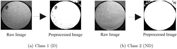
Images of Defective (D) and non-defective (ND) of product 2 before and after preprocessing method (17, 0, 34): (a) Class 1 (D); (b) Class 2 (ND).
Product 3 Manual Preprocessing
Sequence: (17, 14, 0, 3)
The preprocessing sequence applied for Product 3 is (17, 14, 0, 3), corresponding to the following filters and parameters:
-
Low-Pass Filter (17) with a cutoff frequency of 140
-
Robert’s Edge Detection (14)
-
Binarization (0) with a threshold value of 30
-
Enhanced Image (3)
Figure 7 presents the visual outputs of this sequence applied to all three classes.
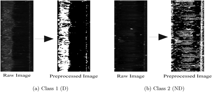
Images of Defective (D) and non-defective (ND) of product 3 before and after preprocessing method (17, 14, 0, 3): (a) Class 1 (D); (b) Class 2 (ND).
Genetic algorithm-based preprocessing optimization
The genetic algorithm framework implements advanced evolutionary computation principles for automated pipeline preprocessing optimization, addressing the computational complexity and interdependency challenges inherent in manual optimization approaches. The genetic algorithm incorporates sophisticated mechanisms that include elitism, multi-objective fitness evaluation, and adaptive genetic operators to ensure robust convergence toward optimal preprocessing configurations37,38,39. Table 3 summarizes the complete set of hyperparameters governing the genetic algorithm, including the core evolutionary operators, advanced elitism settings, and sequence structure constraints employed throughout the optimization process (Fig. 8).

Workflow of genetic algorithm.
Chromosome Encoding and Representation The genetic algorithm employs variable-length chromosome encoding to represent tunable complexity preprocessing sequences. Each chromosome C encodes a preprocessing pipeline consisting of a sequence of filter operations:
$$\begin{aligned} C = \left\{ (f_{k_1}, \varvec{\theta }_1), (f_{k_2}, \varvec{\theta }_2), \ldots , (f_{k_L}, \varvec{\theta }_L) \right\} \end{aligned}$$
(1)
where:
-
\(L \in [L_{\min }, L_{\max }]\) denotes the variable sequence length, with \(L_{\min } = 3\) and \(L_{\max } = 7\) defining the minimum and maximum number of filtering operations
-
\(f_{k_i}\) represents the i-th filter operation, encoded as an integer index \(k_i \in \{0, 1, \ldots , 47\}\) corresponding to the comprehensive library of 48 distinct preprocessing operations, including morphological operations, frequency domain filters, edge detection, smoothing, thresholding, and adaptive enhancement techniques
-
\(\varvec{\theta }_i = [\theta ^{(1)}_i, \theta ^{(2)}_i, \ldots , \theta ^{(m)}_i]^T\) is the parameter vector for filter \(f_{k_i}\), where each parameter \(\theta ^{(p)}_i\) is a real-valued variable normalized to a specified range \([\theta ^{\min }_i, \theta ^{\max }_i]\) determined by the filter’s operational constraints
This variable-length encoding enables the genetic algorithm to explore preprocessing pipelines of different complexities, allowing evolution to discover optimal trade-offs between feature enhancement, computational cost, and classification robustness across diverse defect types.
Population Initialization Strategy
The genetic algorithm initializes the population through random generation, creating 100 individuals where each individual represents a filter sequence. Each sequence is randomly generated by uniformly selecting filter IDs from the 48 available preprocessing filters and randomly assigning parameter values within their valid ranges. The sequence length for each individual is also randomly determined between the minimum (3 filters) and maximum (6 filters) constraints, ensuring diversity in chromosome structure. This random initialization approach ensures comprehensive exploration of the solution space while preventing bias toward any particular filter combination. The population size of 100 individuals provides adequate genetic diversity while maintaining computational feasibility. Using randomness in filter selection, parameter initialization, and sequence length, the algorithm establishes a diverse starting population that enables an effective evolutionary search for optimal preprocessing pipelines in defect detection40,41.
Elitism Mechanism for Solution Preservation
The genetic algorithm incorporates elitism as a fundamental mechanism to preserve the best-performing preprocessing sequences across generations, preventing the loss of high-quality solutions during the stochastic evolutionary process. Elitism ensures that a predetermined number of elite individuals (typically 5-10% of the population size, corresponding to 5-10 individuals) are directly transferred to the next generation without undergoing crossover or mutation operations.
The implementation of elitism follows established principles in which elite individuals are selected based on their fitness rankings and copied unchanged to the subsequent generation. This strategy serves multiple critical functions:
-
Convergence acceleration by maintaining reference points for promising search space regions
-
Preservation of solution by preventing the degradation of optimal preprocessing configurations through genetic operations
-
Convergence monitoring by tracking the best fitness values across generations to detect optimization plateaus
Elite Selection Strategy: Elite selection employs a fitness-based ranking, where the top performers are identified through a fitness score comparison and are systematically preserved. The elite preservation mechanism selects the best \(\varepsilon\) individuals from the current population, where \(\varepsilon = 0.05 \times {population}\_size\) (e.g. 5 individuals from 100), ensuring balanced exploitation of high-quality solutions while maintaining population diversity. The elitism strategy addresses the fundamental trade-off between exploitation and exploration by preserving proven solutions while allowing continued search through the remaining population. This approach prevents the common problem of losing optimal solutions due to the stochastic nature of selection, crossover, and mutation operations.
Crossover operations implement specialized techniques for variable-length chromosomes applied only to non-elite individuals: single-point crossover (probability Pc = 0.8) for filter sequence exchange and uniform crossover (Pc = 0.2) for parameter mixing. Elite individuals bypass crossover operations entirely, ensuring that their optimal configurations remain intact across generations.
Mutation Strategies: Mutation strategies incorporate multiple mechanisms applied exclusively to non-elite offspring: filter replacement mutation (probability \(P_m = 0.08\)) randomly replaces filters with alternatives from the library; parameter mutation (\(P_m = 0.2\)) applies Gaussian perturbation (\(\sigma = 0.1\)) to parameter values; and sequence length mutation (\(P_m = 0.02\)) adds or removes filters from preprocessing sequences. The elitism mechanism protects high-quality solutions from potentially destructive mutations while allowing continued exploration through the remaining population.
Elitist Replacement Strategy: The genetic algorithm implements an evolutionary strategy \((\mu + \lambda )\) where elite individuals from the parent generation compete with newly generated offspring for survival positions. This approach ensures that elite solutions are only replaced if superior alternatives are discovered, maintaining a monotonic improvement in the overall quality of the population.
$$\begin{aligned} \textit{fitness}(C) = \alpha \cdot \text {Accuracy}(C) + (1-\alpha ) \cdot \left( 1 – \text {Norm}_{\text {CompCost}}(C)\right) \end{aligned}$$
(2)
In Equation (2), \(\text {Accuracy}(C)\) denotes CNN classification accuracy on the validation data set obtained from the test model, while \(\text {Norm}_{\text {CompCost}}(C)\) represents the normalized computational cost, including preprocessing and inference time, scaled to the range [0,1]. In this article, the weighting parameter \(\alpha\) is set to 0.7, balancing the trade-off between accuracy and computational efficiency and effectively prioritizing model accuracy while still accounting for computational cost. This bi-objective formulation ensures that the evolved preprocessing sequences are accurate and computationally practical for industrial deployment, facilitating meaningful comparisons of accuracy and inference time in the experimental results.
The replacement mechanism operates as follows: (1) elite individuals are automatically preserved in the next generation, (2) remaining population slots are filled through competitive selection between non-elite parents and all offspring, and (3) fitness-based ranking determines final population composition while maintaining the predetermined elite count.
Convergence and Termination Criteria: Algorithm termination employs multiple criteria to ensure optimal solution convergence while preventing excessive computational overhead: maximum generation limit (150 generations), fitness improvement threshold (<0.001 over 15 consecutive generations), and maintenance of population diversity through genotypic distance monitoring. The elitism mechanism contributes to the stability of convergence by providing consistent high-quality reference points throughout the evolutionary process.
Convergence analysis incorporates statistical testing for fitness stagnation using the elite population subset, where consistent elite fitness values indicate algorithm convergence toward optimal preprocessing configurations. The elitism mechanism enables reliable convergence detection by maintaining stable performance benchmarks across generations.
This comprehensive integration of elites ensures that the genetic algorithm maintains optimal preprocessing solutions while continuing to explore the search space for potentially superior alternatives, balancing the exploitation and exploration requirements essential for effective evolutionary optimization in image preprocessing applications.
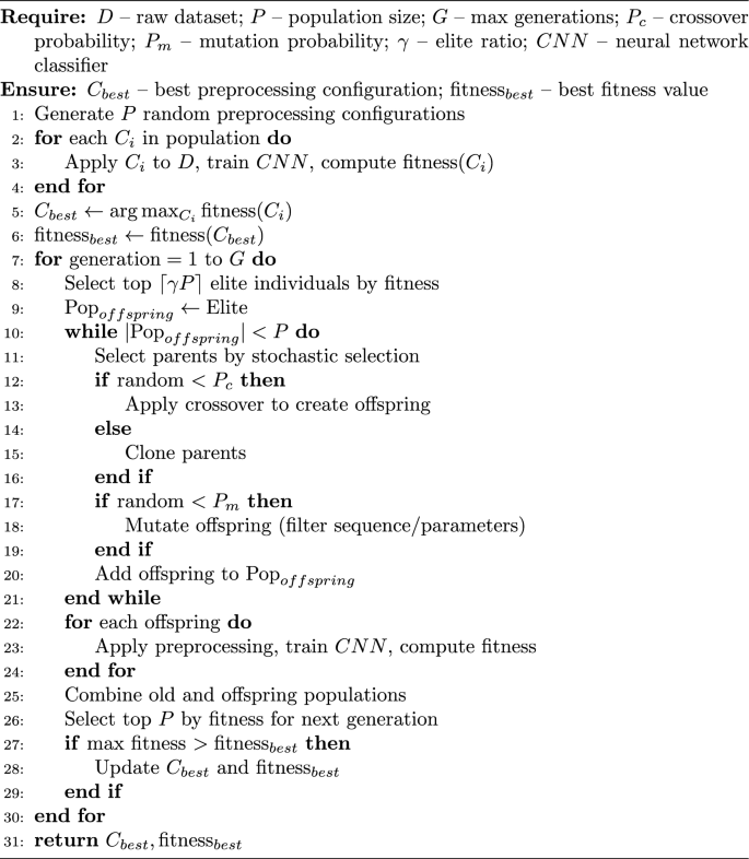
Genetic algorithm for image preprocessing optimization.

Evolution of CNN accuracy across generations for Product 1.

Evolution of CNN accuracy across generations for Product 2.

Evolution of CNN accuracy across generations for Product 3.
The graphs provided in Figs. 9, 10, 11 illustrate the evolution of CNN accuracy across generations for genetic algorithm-optimized preprocessing sequences of varying length (3 to 6 filters), evaluated on three different products. For each product, the genetic algorithm rapidly identifies effective filter sequences, with the best-performing configurations achieving significant accuracy improvements within the first 10–15 generations, demonstrating strong convergence behavior. Notably, shorter sequences (3 or 4 filters) often reach optimal or near-optimal accuracy more quickly, whereas longer sequences may require more generations, but sometimes yield incremental gains for more complex datasets.
In Product 1 (Fig. 9) and Product 3 (Fig. 11), several sequence lengths achieve perfect or near-perfect accuracy, while Product 2 (Fig. 10) shows clearer separation between different sequence lengths, highlighting the importance of tuning pipeline complexity to the underlying data. The stability and consistency of the accuracy plateaus across generations reflect the robustness of the genetic algorithm in preserving high-quality solutions through elitism and selection mechanisms. In all cases, the best evolved sequence for each length maintains its performance in later generations, indicating the effectiveness of the algorithm to retain and refine optimal preprocessing strategies over time. These results collectively emphasize the adaptability and efficiency of the genetic algorithm in discovering sequence configurations that maximize neural network performance for diverse industrial image analysis tasks.
Computational Cost of GA Optimization
To quantify the computational overhead associated with the evolutionary search process, the total execution time required for the Genetic Algorithm to converge on an optimal preprocessing pipeline was systematically recorded. Across five independent runs, the average computational cost for the GA optimization phase was \(391.01 \pm 45.33\) minutes for Product 1, \(90.51 \pm 34.13\) minutes for Product 2, and \(221.55 \pm 51.38\) minutes for Product 3, where the values are reported as mean ± standard deviation. The variance in total computational time across product categories is primarily attributable to the structural complexity of the defects and the resulting length of the dynamically generated filter sequences required to maximize the fitness function. All GA optimization processes–including population initialization, fitness evaluation, and evolutionary operations–were executed using the hardware and software specifications detailed in Table 4. While the initial offline computational cost of the GA search may be higher or lower than that of manual trial-and-error selection, this represents a one-time, upfront investment. Once the optimal preprocessing sequence is identified, runtime inference during active deployment is highly efficient, as demonstrated by the superior test-phase inference times reported in Section 4.
Confusion Matrix The confusion matrix is a widely used tool in machine learning and statistical analysis to evaluate the performance of classification models48,49. Provides a tabular representation of the true labels versus the predicted labels generated by the model. The matrix is particularly helpful for understanding errors made by the classifier and can be used for binary or multiclass classification tasks50,51. For a binary classification problem:
-
True Positives (TP): Correctly predicted positive instances.
-
True Negatives (TN): Correctly predicted negative instances.
-
False Positives (FP): Incorrectly predicted positive instances (type I error).
-
False Negatives (FN): Incorrectly predicted negative instances (type II error)52.
Advantages of genetic algorithm optimization
-
Global Search Capability: Explores multiple solution regions simultaneously, avoiding local optima through population diversity and stochastic operators.
-
Automated Parameter Selection: Eliminates manual preprocessing parameter tuning, reducing expert dependency, and enabling automatic filter sequence optimization.
-
Multi-Objective Optimization: Simultaneously optimizes detection accuracy, computational efficiency, and robustness through weighted multi-objective fitness functions.
Limitations of genetic algorithm optimization
-
High Computational Cost: Requires extensive resources for fitness evaluations across populations, significantly increasing processing time and hardware requirements.
-
Premature Convergence Risk: May converge to suboptimal solutions when genetic diversity is lost, providing no theoretical optimality guaranties.
-
Parameter Sensitivity Issues: Performance is highly dependent on control parameter settings, requiring extensive experimentation and domain expertise for optimization.
Sequences generated by genetic algorithm
In the process of optimizing the preprocessing pipelines with a genetic algorithm, a diverse set of candidate sequences was automatically generated, ranging from three-filter to six-filter configurations. The filters available for selection are listed in Table 2, while their corresponding parameter bounds (lower and upper limits) are defined in the YAML-style configuration provided in the Appendix. This approach allowed the GA to rigorously explore a wide range of filter combinations and parameter settings, maximizing the search for sequences that best fit the neural network in defect detection. Each sequence was evaluated using a robust fitness function that emphasizes classification performance and operational efficiency, ensuring that both precision and practical applicability were considered during selection.
From the collection of candidate sequences, the final sequence chosen for detailed comparison is the one that demonstrated the highest validation accuracy during the evolutionary optimization process. This selection strategy ensures that the reported results represent the optimal achievable benefit of automated pipeline optimization for the respective data set and model architecture. By presenting the highest-performing sequence, the analysis highlights the effectiveness of the genetic algorithm in adaptively identifying preprocessing strategies that outperform standard or manually tuned pipelines, providing a meaningful benchmark for industrial machine vision applications.
Product 1
Sequence: (37, 42, 33, 0, 3, 40)
The Earliest best preprocessing sequence for Product 1 was found in generation 34, 6-filter sequence(37, 42, 33, 0, 3, 40), corresponding to the following filters and parameters:
-
histogram qualification (37)
-
gaussian filter(42) with a sigma value of 3.931298600338181
-
closing operation (33) with a Kernel size of 3
-
Binarization (0) with a threshold value of 165
-
Enchanced image (3)
-
median filter (40) with a Kernel size of 9
Product 2
Sequence: (16, 0, 6)
The Earliest best preprocessing sequence for Product 1 was found in generation 3, 3-filter sequence(16, 0, 6), corresponding to the following filters and parameters:
Product 3
Sequence: (0, 6, 42)
The Earliest best preprocessing sequence for Product 1 was found in generation 1, 3-filter sequence(0, 6, 42), corresponding to the following filters and parameters:
Neural network modelling
A neural network is a computational system inspired by the structure and function of the human brain. It consists of layers of interconnected nodes (neurons) that process data through weighted connections. Neural networks are particularly effective in tasks that require pattern recognition, such as image classification, object detection, and speech recognition. In this research, a convolutional neural network (CNN) was used due to its suitability for image-related tasks. CNNs are specifically designed to process and analyze visual data by leveraging spatial hierarchies in images42,43. This study used two sets of images: the original images and the preprocessed images. The preprocessed images were generated using three distinct preprocessing methodologies (Fig. 12).

The flowchart to implementation of the CNN model.
For each configuration, the individually trained models were evaluated to determine the accuracy achieved and the minimum number of images required to achieve satisfactory training for both the original and preprocessed images. Furthermore, the results were analyzed to compare the performance of models trained with different preprocessing sequences with those trained on the original images.
Convolutional neural network (CNN)
Convolutional Neural Networks (CNNs) are widely used for image analysis and defect detection due to their ability to automatically extract hierarchical features from images44,45. The complete architecture and training configuration of the model are summarized in Table 5. Applying convolutional layers, CNNs detect edges, textures, and patterns, making them highly effective for classification and anomaly detection tasks. The network is trained on labeled datasets, allowing it to learn optimal feature representations and improve accuracy over time. When integrated with optimized preprocessing techniques, CNNs improve defect recognition by focusing on the most relevant image features while minimizing noise and artifacts.
Evaluation metrics
The evaluation of the neural network model is performed using a set of key parameters that provide information on the performance and efficiency of the model. These parameters play a crucial role in deciding the best order of the preprocessing steps and determining the number of images needed to ensure successful model training. Metrics such as accuracy, sensitivity, specificity, precision, execution time, memory usage, and the confusion matrix are systematically analyzed to assess the model’s ability to achieve reliable and efficient results46,47. By carefully examining these metrics, it becomes possible to identify the most suitable preprocessing pipeline and the ideal data set size for training, ensuring that the model achieves optimal performance while maintaining computational efficiency. This structured evaluation process is critical for selecting the best configuration for specific applications and use cases.