Modeling of scour hole characteristics under turbulent wall jets using machine learning

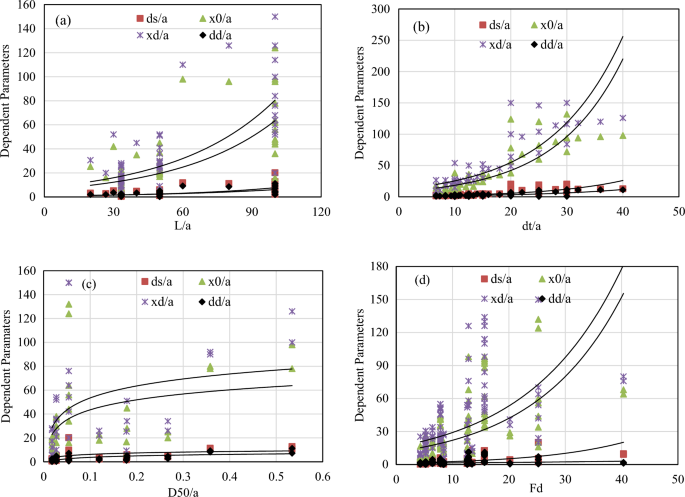
Considering all the necessary data for the analysis, both multiple linear regression analysis (MLRA) and non-linear multiple regression analysis (MLRA) are performed. The nondimensional dependent variables considered in this study are maximum equilibrium scour depth \(\left({d}_{s}/a\right)\), the distance to scour depth from the end of rigid apron \(\left({x}_{0}/a\right)\), the height of dune \(\left({d}_{d}/a\right)\) and the distance to maximum height of dune crest from the end of rigid apron \(\left({x}_{d}/a\right)\). From Gamma test, densimetric Froude number (F_d), apron length (L), tail water level (d_t), median sediment size (D₅₀) are found to be influencing these four dependent parameters. For modelling, apron length (L), tail water level (d_t) and median sediment size (D₅₀) are made dimensionless numbers by dividing them with height of gate opening (a) such as L/a, d_t/a, D₅₀/a respectively. The results of variation of dependent parameters with input parameters are analyzed as demonstrated in Fig. 4a–d. Present research reports a rising trend between all dependent parameters against the apron length (L/a), as shown in Fig. 4a. The reason for this trend is attributable to the dissipation of energy of the jet as it travels over the apron. Hence, longer aprons are able to dissipate larger energy and reduce the erosive capacity of the jet. Similarly, rising trends are also visible for the variations of dependent parameters with tail water level (D_t/a), densimetric Froude number (F_d), and median sediment size (D₅₀), as shown in Fig. 4.

A number of single regressions models for maximum equilibrium scour depth \(\left({d}_{s}/a\right)\), the distance to scour depth from the end of rigid apron \(\left({x}_{0}/a\right)\), the height of dune \(\left({d}_{d}/a\right)\) and the distance to maximum height of dune crest from the end of rigid apron \(\left({x}_{d}/a\right)\) with different input parameters are established. After rigorous study, the best models for each couple (dependent vs independent) with high coefficient of determination R² are identified. Then, multiple regression analysis has been performed and two equations (one for linear and another for nonlinear cases) are obtained for each dependent parameter, as provided below.

Resulted equations from multiple linear regression analysis (MLRA)

MLRA for maximum equilibrium scour depth \(\left({d}_{s}/a\right)\)

MLRA for distance to scour depth from the end of rigid apron \(\left({x}_{0}/a\right)\)

MLRA for distance to maximum height of dune crest from the end of rigid apron \(\left({x}_{d}/a\right)\)

MLRA for the height of dune \(\left({d}_{d}/a\right)\).

Resulted equations from multiple non-linear regression analysis (MNLRA)

MNLRA for maximum equilibrium scour depth \(\left({d}_{s}/a\right)\)

MNLRA for distance to scour depth of from the end of rigid apron \(\left({x}_{0}/a\right)\)

MNLRA for the distance to maximum height of dune crest from the end of rigid apron \(\left({x}_{d}/a\right)\)

MNLRA for the height of dune \(\left({d}_{d}/a\right)\)

The coefficient of determination R² for multiple linear regression equation and multiple nonlinear regression equation are found to be 0.56 for \(\frac{{d}_{s}}{a}\), 0.66 for \(\frac{{x}_{0}}{a}\), 0.67 for \(\frac{{x}_{d}}{a}\), 0.56 for \(\frac{{d}_{d}}{a}\) and 0.66 for \(\frac{{d}_{s}}{a}\), 0.74 for \(\frac{{x}_{0}}{a}\), 0.74 for \(\frac{{x}_{d}}{a}\), 0.54 for \(\frac{{d}_{d}}{a}\) respectively which measures the percentage of how much of the total variance is explained by the independent variables. Further, an attempt has been made to apply two machine learning approaches such as ANN-PSO and GEP to model these four parameters \({d}_{s}/a\), \({x}_{0}/a\), \({d}_{d}/a\) and \({x}_{d}/a\).

Model development using ANN-PSO

In this ANN-PSO modelling, several trials were performed and the coefficients C₁ and C₂ were fixed at 1 and 2.5, 2 and 2.5, 1.5 and 2.5, 1.5 and 2.5 for \({d}_{s}/a\), \({x}_{0}/a\), \({d}_{d}/a\) and \({x}_{d}/a\) respectively. The error analysis results for the training data, testing data, and the entire dataset for various swarm sizes and number of neurons (N) for each dependent parameter were analysed. It was observed that the swarm size increases with the same values of C₁ and C₂. While maintaining the number of neurons constant, the values of R², E, and I_d decrease, while the value of RMSE increases.

Model development using GEP

In this section, model development for four dependent parameters using the GEP approach is described. By incorporating all the four independent input parameters (L/a, d_t/a, D₅₀/a, F_d), GEP expression has been derived and GeneXpro Tools 5.0 software package is used for this analysis. Using normalized data, four attempts have been made with the variation of chromosome number, fitness function, and number of runs for modelling the wall jet scouring. Table 6 shows the corresponding parameters of the optimized GEP model.

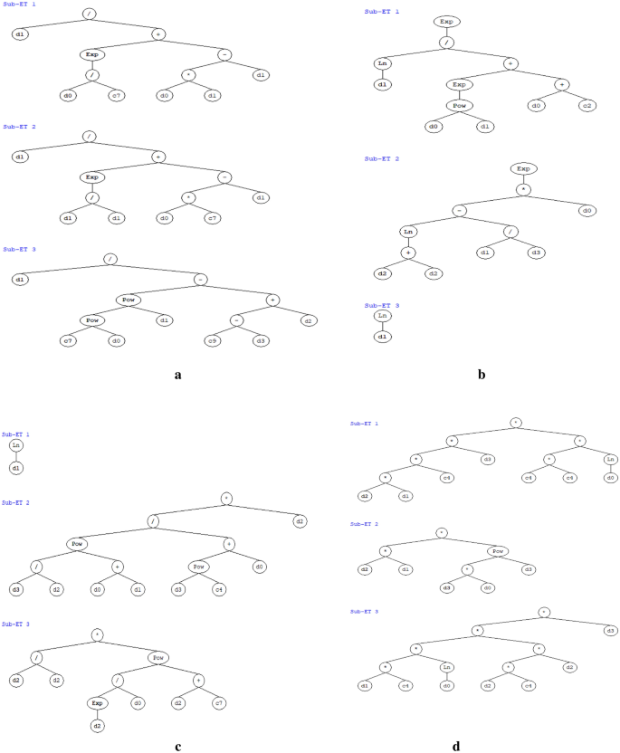
The expression trees for models of \({d}_{s}/a\), \({x}_{0}/a\), \({d}_{d}/a\) and \({x}_{d}/a\) are presented in Fig. 5a–d, respectively. In this expression tree, d₀ = L/a, d₁ = d_t/a, d₂ = D₅₀/a and d₃ = F_d. In Sub-ET 1, 2 and 3 (Fig. 5a), C₇ and C₉ are constants, and their values are 3.45 and − 5.56 respectively for model of \({d}_{s}/a\). In Sub-ET 1 (Fig. 5b), C₂ is constant, the value is − 8.93 for model of \({x}_{0}/a\). In Sub-ET 2 and 3 (Fig. 5c), C₄ and C₇ are the constants, and their values are 2.971 and − 0.376 respectively for model of \({x}_{d}/a\). In Sub-ET 1 and 3 (Fig. 5d), C₄ is constant, the value is − 3.114 and 3.145 respectively for model of \({d}_{d}/a\). The equations derived from the expression trees are presented in Eqs. (16)–(19).

Expression for \({d}_{s}/a\):

Expression for \({x}_{0}/a\):

Expression for \({x}_{d}/a\):

Expression for \({d}_{d}/a\):

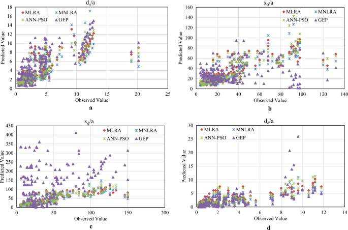
Figure 6a–d shows the relationship between observed and predicted values for the model of \({d}_{s}/a\), \({x}_{0}/a\), \({x}_{d}/a\) and \({d}_{d}/a\) respectively. It is observed that the predicted model of ANN-PSO gives good agreement with observed values for all the four models, whereas GEP shows the unsatisfactory result of the present study.

Performance of uncertainty and reliability analysis

To perform a comprehensive statistical assessment of the proposed models, two indices namely confidence interval (U95) and reliability index are computed. The statistical evaluation of the present models, highlighting their predictive capabilities and robustness using uncertainty analysis and reliability index, is presented in Table 7.

Table 7 shows the confidence interval (U95) and reliability index (RI) of MLRA, MNLRA, ANN-PSO and GEP in predicting \({d}_{s}/a\), \({x}_{0}/a\), \({x}_{d}/a\) and \({d}_{d}/a\). ANN-PSO model represented the lowest values of confidence interval (U95), i.e., 0.383, 2.539, 2.805 and 0.268 when compared to MLRA (0.402, 2.604, 3.101and 0.293), MNLRA (0.415, 2.598, 3.063 and 0.301) and GEP (0.483, 28.800, 19.276 and 0.409) for predicting \({d}_{s}/a\), \({x}_{0}/a\), \({x}_{d}/a\) and \({d}_{d}/a\) respectively. Additionally, predictions of \({d}_{s}/a\), \({x}_{0}/a\), \({x}_{d}/a\) and \({d}_{d}/a\) provided by ANN-PSO are more reliable (RI = 0.573, 0.591, 0.576 and 0.548) when compared to other present models. Moreover, MNLRA shows slightly less reliable (RI = 0.521, 0.545, 0.570 and 0.497) than ANN-PSO in predicting \({d}_{s}/a\), \({x}_{0}/a\), \({x}_{d}/a\) and \({d}_{d}/a\). GEP shows wider confidence intervals (U95) and lower relative index, indicating higher uncertainty and less reliable model in predicting \({d}_{s}/a\), \({x}_{0}/a\), \({x}_{d}/a\) and \({d}_{d}/a\). This analysis suggests that the ANN-PSO provides a more consistent and reliable model for the prediction of \({d}_{s}/a\), \({x}_{0}/a\), \({x}_{d}/a\) and \({d}_{d}/a\).

Statistical error analysis

This section illustrates the performance of the two soft-computing models and two multiple regression models in predicting \({d}_{s}/a\), \({x}_{0}/a\), \({x}_{d}/a\) and \({d}_{d}/a\). To assess the strength of present approaches, seven statistical indices are accounted including two statistical indices such as Root mean square error (RMSE) and coefficient of determination (R²), and two relative indices, E and I_d^{38,49,50,51,52}. The error indices are computed for all the present models in terms of MAE, MAPE, MSE, RMSE, R², E and I_d are depicted in Table 8.

From Table 8, it is found that for both \(\left({d}_{s}/a\right)\) and \(\left({x}_{0}/a\right)\), the error indices, i.e., MAE, MAPE, MSE and RMSE are less for MLRA and MNLRA as compared to the ANN-PSO and GEP. But, the error indices, i.e., MAE, MAPE, MSE and RMSE are found to be less for ANN-PSO as compared to MLRA, MNLRA and GEP for both \({x}_{d}/a\) and \({d}_{d}/a\). However, the R² value is more in ANN-PSO model for all predicting parameter values. E and Id values are also found to be close to 1 for ANN-PSO models for all three predicting parameter values except \(\left({x}_{0}/a\right)\). For \(\left({x}_{0}/a\right)\), E and Id values are found to be close to 1 for MLRA model. By comparing all the statistical parameters, ANN-PSO model shows better result as compared to the other presented regression and soft computing techniques (Table 8).