Data
Data were derived from the Medical Birth Register (MBR) which covers around 98% of all births in Sweden and was established in 197319. Data from ante-, intra- and perinatal care are collected prospectively by the National Board of Health and Welfare (NBHW)19. Through the unique personal identification number (PIN)20 data in the MBR is linked with the Cause of Death Register, the Patient Register for inpatient and outpatient specialized care (main and secondary diagnoses are coded according to the Swedish version of the ICD-system 10th revision since 199819 and the Prescribed Drug Register (established 1952, 1964 and July 2005, respectively)19,20,21,22,23 at the NBHW.
The years included in the respective linked registers are summarized in Table S6 in the supplementary material. Table S7 in the supplement displays the register origin of each variable (outcomes and predictors) considered in the analysis19. Five used variables (mode of delivery, gestational length at birth, preeclampsia, preexisting chronic hypertension and preterm prelabour rupture of the membranes) have already been defined in previous studies24,25,26 based on existing variables in the MBR (Table S1, S8).”
Participants
The initial study population consisted of nulliparous women across all registered age groups with a low-risk pregnancy who gave birth in Sweden at or beyond 41 + 0 GW between 1998 and 2019. Low-risk was defined as having a singleton fetus in cephalic presentation, no gestational or preexisting diabetes (Type 1 or 2) and an antenatal hospital admission not longer than five days before birth (Fig. 1a, Fig. S1 supplementary material). Pregnancies with known risk-factors are generally induced earlier than 41 + 0 GW.
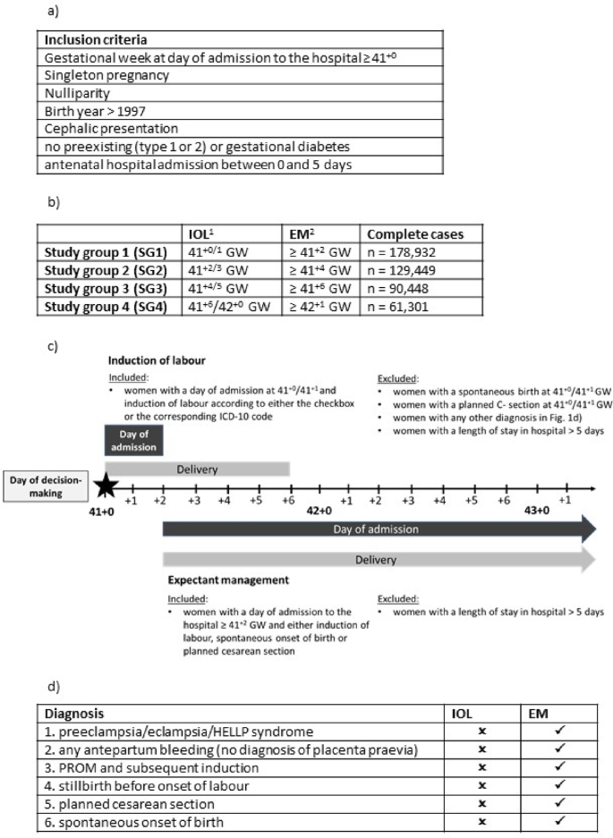
Design of the study population and the study groups 1-4. (a) Inclusion criteria applied to all registered pregnancies between 1992-2019. (b) Design of the study groups based on the study population. 1Induction of labour registered either through checkbox o corresponding ICD-10 code. The gestational age corresponds to the gestational age at the day of admission to the hospital. 2Later onsets of labour than the induced women in the respective group, including later IOL, planned cesarean and spontaneous birth. (c) Construction of study group 1 and the corresponding binary variable “induction of labour”. (d) 1.−4.: The most common diagnosis leading to an induction of labour (“confounding by indication”). Pregnancies with these diagnoses were excluded in the respective induction of labour group, while not in the respective expectant management group. Other onsets of labour (5 and 6) at the same gestational age as the induced women were excluded in respective study group. IOL: induction of labour. EM: expectant management. GW: gestational weeks. HELLP-Syndrom: acronym for hemolysis, elevated liver, low platelet counts. PROM: premature rupture of the membranes.
We modified the inclusion criteria in the initial study population to reflect clinical decision-making and routines as well as for comparability to previous research from RCTs and observational studies7,8,9,27,28. Obstetricians and women usually decide during a consultation based on the medical findings if the pregnancy should be induced or not (referred to as day of decision-making). Study group 1 included women who were induced at 41+0– 41+1 (referred to as IOL) and women who delivered beyond 41+1 irrespective of onset of labour, i.e. elective cesarean delivery, IOL or spontaneous onset (referred to as EM). Women who delivered spontaneously, including premature rupture of the membranes (PROM) and subsequent induction, or by elective cesarean section at 41+0– 41+1 were excluded for Study group 1. In total, four different study groups (SG) were constructed, depending on gestational length and timing of IOL; SG1: IOL 41+0– 41+1 and EM > 41+1, SG2: IOL 41+2−41+3 and EM > 41+3, SG3: IOL 41+4−41+5 and EM > 41+5; SG4: IOL 41+6−42+0 and EM > 42+0 (Fig. 1b and c, Fig. S6 supplementary material).
The timing of IOL was calculated by using the gestational age at the day of admission to the hospital as a proxy (see section “Data preparation”) since the MBR does not provide the exact day of induction. Under clinical assumptions it is very unlikely that a woman at such a late stage of pregnancy (≥ 41 GW) is admitted to hospital without any intervention or giving birth (Fig. 1c, Fig. S6 supplementary material).
Women in each IOL group who had one of the following diagnoses registered were excluded to ensure that these women were only induced because of gestational age, not because of an underlying pathology: Hypertensive pregnancy disorders (Preeclampsia, eclampsia, HELLP-Syndrome), IUFD (intrauterine fetal death) or any antepartum bleeding (without a diagnosis of placenta previa) (Fig. 1d). Women with these diagnoses were not excluded in the corresponding EM group.
Data preparation
The majority of variables are directly transferred to the NBHW from the standardized clinical records, where the information is generally collected through pre-specified checkboxes or through assigned diagnostic or procedure codes19. At the NBHW, the records are merged, quality checked, and annually released for the use as the MBR19.
The data-preprocessing steps conducted by the authors of the present study were to create the study population (see “Participants”) and the predictors. Variables for “gestational age at day of admission to the hospital”, “length of antenatal stay in hospital” (directly before birth), “onset of labour” and decision on IOL or EM (“induction of labour”) were created.
“Gestational age at the day of admission to the hospital” was calculated based on the existing variables “gestational age at delivery”, “birth date of the infant” and the “day of admission to the hospital”. The difference between the “birth date of the infant” and the “day of admission to the hospital” is the “length of antenatal stay in hospital” in days. In a second step the values for “length of antenatal stay in hospital” were subtracted from “gestational age at delivery” which resulted in the “gestational age at admission to the hospital”.
Onset of labour (elective cesarean, induction of labour or spontaneous onset) was classified hierarchically based on a checkbox for labour onset and a corresponding registered ICD-10 diagnosis (Table S1 Supplementary material). A premature rupture of the membranes with a subsequent induction of labour was classified as a spontaneous onset of labour (Table S1 supplementary material).
The binary variable “induction of labour” in the respective study group (SG1-SG4) was based on “gestational age at day of admission to the hospital” and “onset of labour”. Women classified as IOL in the respective group (Fig. 1b and c, Fig. S6 supplementary material) were the positive class and women who were classified as EM were the negative class.
Dimension reduction was done for smoking and snuff use. The three existing self-reported variables on smoking before, in early and late pregnancy with four categories (unknown, no smoking, 1–9 cigarettes/day, ≥ 10 cigarettes/day) were combined into two variables (smoking before and during pregnancy) with three categories (yes/no/unknown) (Table 1). Those, who smoked at any time during pregnancy were categorized as smoking during pregnancy.
Outcomes
The main outcomes of the study were mode of delivery categorized into cesarean section, vaginal operative delivery (forceps or ventous) and spontaneous vaginal birth. Each outcome was predicted separately (no composite outcome).
Predictors
To ensure a predictive design with a potential for prospective use, only variables which are known at the day of decision-making regarding IOL in each study group (Fig. 1c) were used as features (Table 1). These features included diagnoses of some diseases which did not meet the exclusion criteria of the study (asthma, antepartum bleeding, epilepsy, chronic hypertension, nephrological disease, systemic lupus erythematosus, inflammatory bowel disease, urinary tract infection), as well as pregnancy-related variables (decision on IOL or EM, antepartum PROM, assisted reproduction, number of antenatal visits in antenatal care, self-reported number of previous spontaneous miscarriages, number of years of involuntary childlessness, smoking/snuff use before or during pregnancy, and mother’s height, weight and BMI at first antenatal visit) and sociodemographic predictors (mother’s country of birth, father’s citizenship, family situation). All non-binary categorical variables were one-hot encoded resulting in n = 43 features used in the prediction models. Diagnoses and clinical characteristics which occurred later (i.e. during expectant management) or during labour were not considered.
Missing data
Missing values for the included variables range over time but rarely exceeds 5–10% with a further decreasing trend since the start of the digitalized report to the NBHW in 200719,29.
In the present study population missing values did not exceed 5% beside body mass index (BMI) and smoking/snuff use (Table 1, Table S2 supplementary material). Missing values were treated according to the mechanism why they were missing (e.g. missing completely at random, missing at random, missing not at random). We classified BMI as missing not at random. It cannot be ruled out that mother’s pre-pregnancy BMI is calculated only when overweight or obesity is obvious30, as well as technical issues29. The rate of missing values of maternal pre-pregnancy height are below 5% (Table 1) and the validity is considered high19. However, the rate of missing values for BMI before imputation in the four study groups ranged between 8.3 and 8.5% (data not shown). BMI was imputed by using mother’s height from a next pregnancy registered in the MBR during the included time-period, which decreased the rate of missingness to 7.7–7.8% (Table 1.)
We also considered the variables smoking and snuff use to be missing not at random. Although the validity of the information on smoking is high, there is evidence on relevant underreporting of active smoking in early and late pregnancy by self-reported quitters31. Assuming that women start smoking (using snuff) during pregnancy very rarely29, missing values were replaced based on the values registered at other time points, i.e. smoking before, in early or late pregnancy (Table S2 supplementary material). The remaining missing values (e.g. values for smoking before pregnancy were not registered before 1999) were summarized in the category “unknown” (Table 1).
Introducing a category “unknown” for categorical variables reflects the nature of register data as well as the clinical setting and is in line with the literature11. This was also applied for the variables for mother’s country of birth and father’s citizenship (Table 1).
An exception in the registers are the diagnoses which are registered by checkboxes. In these cases, there is only a registered value, if the respective diagnosis is present. No missing values can be calculated. The usual procedure for variables based on checkboxes is to replace missing values with zero (no event occurred).
Another exception are the variables “number of previous spontaneous abortions” and “years of involuntary childlessness”, which are self-reported. Zero values (no event occurred) are not registered. For descriptive analysis the missing values were not considered and the mean was only calculated for those women who reported at least one event (Table 1). For the machine learning analyses, the missing values were replaced by zero, meaning that no such event occurred. Similar to the checkboxes, no amount of missingness could be calculated.
For the creation of the study population, observations with missing values in some of the variables had to be excluded. However, missing values for the respective variables did not exceed 1,6% (Fig. S1 supplementary material).
Analytical methods
A complete case analysis was conducted in all models. Observations with at least one missing value in the outcome or predictor variables were excluded (Table 1, Fig. S1-S5 supplementary material). Data preprocessing and handling of missing values were the same for all analyses in each study group.
In each study group, five different classifiers (random forest, support vector machine, neural network, mixed naïve bayes and logistic regression) were compared while predicting every chosen outcome in a binary classification. According to the requirements of the respective classifier, continuous variables were standardized with standard scaler (zero mean and unit variance) for logistic regression, support vector machine and neural network.
Additionally, a multiclass classification analysis was conducted using the best-performing classifier from the separate binary outcome evaluations, in order to account for potential inconsistencies or overlaps in the one-vs-rest approach and to assess performance for the mutually exclusive modes of delivery. This approach ensures a single, unambiguous prediction per observation, which better reflects the clinical decision-making task.
The four study groups were randomly split into a training (70%), a validation (10%), and a test (20%) set with stratification for the outcome rate in each analysis (Table S3 supplementary material). Because of the exploratory approach, initially non-tuned analyses with the default values of each classifier were run and presented to have a benchmark comparison.
All steps of the analyses including data-preparation were processed with Python Version 3.10. The code was written using the scikit-learn machine learning library for the support vector machine (linear kernel), random forest (n_estimators = 100, max_depth = None, min_split = 2 as default values in the library) and logistic regression model (penalty = None). TensorFlow open source machine learning framework was applied to build the neural network. The model was constructed with two hidden layers (64 and 32 neurons respectively) using ReLU activation function and one output layer with a single neuron and a sigmoid activation function for binary classifications. After configuration (optimizer = ‘adam’, loss = ‘binary_crossentropy’) the model was trained for 10 epochs. For the multiclass prediction we used the cross entropy softmax activation function (sparse_categorical_crossentropy) in the output layer, appropriate for mutually exclusive classification tasks. All other characteristics of the neural network architecture and training procedure remained the same as in the binary classification setting. We used the mixed-naïve-bayes package for categorical and Gaussian Naïve Bayes32.
Performance metrics
The performance of the models was evaluated by plotting receiver operating characteristic curves (ROC) and precision recall curves (PR) for each outcome in each group. To quantify the performance, the corresponding areas under the curves (auROC, auPR) were calculated with the roc_auc_score function and average_precision_score from scikit-learn. The respective 95% confidence interval (CI) was assessed by applying the RepeatKFold function with 5 splits and 20 repeats (scikit-learn library).
While auROC is measuring how well the respective algorithm is able to distinguish between the positive and the negative class across different thresholds, auPR provides additional information on performance in case of imbalanced data sets. The auPR is a metric for evaluating the prediction of the positive class only.
Calibration curves were additionally plotted to analyze the reliability of the predicted probabilities for each outcome. The curves were plotted by using CalibrationDisplay.from_predictions (scikit-learn library). The package bins the predicted probabilities into n numbers of bins and calculates both the mean predicted probability and the fraction of true positives in each bin. We chose n = 10 bins to depict every 10% of predicted probabilities. To provide more information of the distribution of the predicted probabilities, histograms were plotted which map how often the respective probabilities were predicted throughout the range (0% − 100%).
Sensitivity, specificity, positive predictive value (PPV) and balanced accuracy were calculated at a 50% threshold (default value).
For consistency, the additional multiclass prediction model was evaluated by calculating the same performance metrices as described for the binary outcomes (sensitivity, specificity, PPV, balanced accuracy, auROC, auPR and calibration curves including histograms for predicted probability).
For the support vector machine classifier, performance metrics on a 50% threshold and not auROC or auPR were evaluated as this classifier does not directly provide probability estimates. The values summarized in the classification report were very low (Table S4 supplementary material).