
This section outlines the operational process of the proposed Student Classification System (SCS-B), which utilizes machine learning techniques. The system acquires student information from the Student Questionnaire (SQ). Further, the collected student data is processed with singular value decomposition for dimensionality reduction. And, neural network is used for training and testing the samples for classifying the data under A, B, C and D for providing further actions to improve results.
Methodological framework overview
To ensure methodological transparency, reproducibility, and practical relevance, this section details the end-to-end workflow adopted for developing the behaviour-based student classification system (SCS-B). The study commenced with the administration of a structured and validated Student Questionnaire (SQ), which captured multidimensional data across five core domains: learning strategies, personal demographics, behavioural traits, intellectual capacity, and comprehensive skill sets.
Responses from 200 undergraduate students were collected, digitized, and systematically normalized to mitigate scale-related biases. All categorical and ordinal variables were encoded to be machine-readable for downstream analysis. To reduce noise and high-dimensional sparsity, singular value decomposition (SVD) was employed, serving the dual purpose of outlier detection and dimensionality reduction. The number of retained singular values was empirically determined by preserving at least 95% of cumulative explained variance, ensuring that no critical information was discarded.
Subsequently, the processed dataset was split into training (80%) and testing (20%) subsets. A fivefold cross-validation strategy was implemented to assess the generalizability and stability of the model. For classification, a backpropagation neural network (BP-NN) was deployed, consisting of a single hidden layer, sigmoid activation functions, a learning rate of 0.01, and trained over 100 epochs with a batch size of 16. To enhance the model’s discriminative power and reduce overfitting, a genetic algorithm (GA) was integrated for feature subset selection. The GA operated with a population size of 50, a crossover probability of 0.8, a mutation rate of 0.05, and a fitness function grounded in classification accuracy.
Overall, this multi-stage pipeline ensures a statistically validated, computationally efficient, and educationally interpretable model for behaviour-driven student classification.
SQ based data collection
The major contribution of this work is to collect data using Student Questionnaire. Here, the student data based on various significant features that influences the student performances. In this model, the SQ is framed based on five different factors, as,
-
1.
Learning techniques.
-
2.
Personal information.
-
3.
Student behaviour.
-
4.
Intellectual factors.
-
5.
Comprehensive ability.
Concerning the aforementioned factors, student data is gathered, and a structured questionnaire (SQ) is provided as an example in Table 1. By utilizing the responses obtained from the SQ, a dataset is generated for the purpose of training and testing the neural network (NN).
Process of outlier detection and dimensionality reduction
Here, both outlier detection and dimensionality reduction in the obtained student data set is processed with singular value decomposition. It can be viewed as the transformation of Eigen vector decomposition from a square format to alternative representations. And, the original student data set (SD) is taken here as, \(SD \in {\mathbb{R}}^{a \times b}\), where, ‘\(a\)’ is the number of data samples and ‘\(b\)’ is the number of features that are linked with the samples. After processing with the singular value decomposition, the following orthogonal matrices are framed,
\(A \in {\mathbb{R}}_{a \times a}\) and \(B \in {\mathbb{R}}_{b \times b}\), further, \(SD\) is given as,
In the above equation, the summation operation is performed with the factors that diagonal matrix as \(\sum = \left[ {dia\left( {\mu_{1} , \mu_{2} , \ldots , \mu_{n} } \right), 0} \right]^{T}\) in the case, \(a > b\), here, ‘0’ denotes the zero matrix and ‘\(\mu_{i}\)’ is the singular values of \(SD\) that are presented in sliding order. If the value of zero matrix is negotiated, the related vectors of ‘A’ can also be remover, and hence, \(\sum = dia\left( {\mu_{1} , \mu_{2} , \ldots , \mu_{n} } \right)\) and \(A \in {\mathbb{R}}_{a \times b}\). That is, ‘b’ dimensions co-ordinate model can be defined in the space of inputs whose coordinates are linked to their sample features and the sample of each student from SD is denoted by a point.
When the coordinate sample is \(sd_{i}\), which can be in the row vector of ‘\(SD\)’, then the process of singular value decomposition is given as the transformation of axes in the space. And, the column vector ‘\(b_{i}\)’ of ‘B’ is representing the base vector of new planner factors defined. The newly defined based vectors can be provided the sample connectivity with the sample features. It is also considered the new base vectors are vertical to each other, since, the matrix ‘B’ is orthogonal. Assume,
$$\widehat{SD} = SD B$$
(2)
From the above equation, it can be observed that each row vector \(\widehat{SD}_{i}\) in \(\widehat{SD}\) denotes the new system’s data coordinate. Further, the singular values that connect the various base vectors denote the sample dispersion on those flows. If the values are greater, the dispersion is wider, denotes large amount of data stored.
Outlier detection
In this section, the total divergence is computed by estimating the weight factor. Before computing that, the singular values are sorted in descending order \(\mu_{1} \ge \mu_{2} \ge \cdots \ge \mu_{n}\). The Weight Factor (WF) is calculated as,
$$WF_{j} = \frac{{\mathop \sum \nolimits_{k = 1}^{j} \mu_{k}^{2} }}{{\mathop \sum \nolimits_{k = 1}^{n} \mu_{k}^{2} }}$$
(3)
The sample bias ‘i’ on the new vector ‘\(b_{j}\)’ can be denoted with Z-score (ZS) and the computation is given as,
$$ZS_{ij} = \frac{{\widehat{{sd_{ij} }} – \gamma_{j} }}{{\sqrt {\mathop \sum \nolimits_{k = 1}^{m} \left( {\widehat{SD}_{ij} – \gamma_{j} } \right)^{2} } }}$$
(4)
where ‘\(\widehat{SD}_{ij}\)’ is the factors of ‘\(\widehat{SD}\)’ and ‘\(\gamma_{j}\)’ denotes the average of all factors in column vector \(\widehat{sd}_{j} = \left( {\widehat{sd}_{ij} , \widehat{sd}_{2j} , \ldots , \widehat{sd}_{nj} } \right).\) The total divergence (\(TD_{i}\)) is computed as,
$$TD_{i} = \mathop \sum \limits_{j = 1}^{n} ZS_{ij} WF_{j}$$
(5)
After computing ‘\(TD\)’ for all student samples, a threshold rate (TR) is fixed. When the TD value becomes greater than the TR, it will be deleted. This can improve the prediction accuracy with the consistent training data set.
Dimensionality reduction
In this context, singular value decomposition (SVD) is applied to reduce the dimensionality of the dataset samples. This reduction involves removing the smaller values and their associated vectors from matrices A and B. Further, the matrices are reframed as, \(\sum\nolimits_{1} = dia\left( {\mu_{1} ,\mu_{2} , \ldots ,\mu_{n} } \right)\), \(A^{\prime} \in {\mathbb{R}}_{a \times k}\) and \(B^{\prime} \in {\mathbb{R}}_{b \times k}\), where, ‘k’ denotes the number of retained singulars and the equation can be recreated as,
$$SD^{\prime } = A^{\prime } \sum\limits_{1} {B^{\prime T} }$$
(6)
Moreover, the vector rates with smaller singular values are having high connectivity with the student class, which enhances the precision rate in classification results. For that, the significance score (SS) of the base vector is computed as,
$$SS_{j} = \sqrt {\mu_{j} } \mathop \sum \limits_{i = 1}^{n} \left| {C_{i} } \right|b_{ij}^{2}$$
(7)
where ‘\(C_{i}\)’ is the correction correlation factor between real student features and classes and \(b_{ij}\) is the element of ‘B’, denotes the connectivity between the real student features and new vectors. Further, the fraction of data retained can be given as,
$$Data \; reserved\;fraction = \frac{{\sqrt {\mathop \sum \nolimits_{i = 1}^{k} \mu_{i}^{2} } }}{{\sqrt {\mathop \sum \nolimits_{i = 1}^{k} \mu_{i}^{2} } }}$$
(8)
where ‘k’ denotes the number of retained vectors.
The dimensionality reduction of the student sample space can be reduced the over fitting because of data diversities and enhance the generalization factor of the model. Additionally, the data set noise can vary the results and hence, dimensionality reduction is processed.
To enhance reproducibility and ensure methodological soundness, fixed thresholds used in this study—such as the Z-score threshold for outlier detection and the truncation point in singular value decomposition (SVD)—were selected based on empirical observation and established statistical conventions. A Z-score threshold of 2.5 was adopted to identify extreme deviations from the mean while minimizing false exclusions, which is consistent with standard practice in educational and behavioral data filtering. For dimensionality reduction via SVD, the number of retained singular values was determined based on cumulative explained variance, with a 95% preservation cutoff used to ensure that most of the meaningful variation in the dataset was retained. These values were initially explored through trial runs and refined through fivefold cross-validation, where model performance metrics such as accuracy and generalization error were monitored. Thus, while fixed, these thresholds were not arbitrary but data-driven and optimized for stability across different experimental configurations.
Process of student behaviour analysis
In the section, the student performances and behaviours are analysed by training with the Back Propagation Neural Networks. The training algorithm is combined with Genetic Algorithm for reducing the overfitting. After performing the training process with Neural Networks with better generalization, the significant features are determined using GA. The complete functions involved in the proposed work with flow are presented in Fig. 2.

Work flow of behaviour based student classification system (SCS-B).
Incorporation of NN for training
After performing dimensionality reduction with the student data set, the Back Propagation NN is used for measuring the student behaviours. Here, the student data samples that are collected from questionnaires are given as \(SD^{\prime} \in {\mathbb{R}}_{m \times k}\), where, ‘m’ denotes the number of samples remains after removing the outliers from SD and ‘k’ is the number of retained features. Here, the dataset \(DS = \left\{ {\left( {u_{1} , v_{1} } \right),\left( {u_{2} , v_{2} } \right), \ldots , \left( {u_{m} , v_{m} } \right) } \right\}\), where, \(u_{i} = \widehat{sd}_{i}\) is a row vector of \(SD^{\prime}\) and \(v_{i}\) is the class label of ‘i’ the student sample. The NN contains three layers, in which the first layer is the input layer comprises ‘k’ number of nodes for proving the inputs ‘\(u_{i}\)’ and the output layers are to provide prediction results as ‘\(v_{i}\)’. The middle layer is the hidden layer, which has ‘n’ number of adaptive nodes based on requirements. The node thresholds make the neural network become non-linear and the equivalent function is computed as,
$$\widehat{{v_{i} }} = f\left( {u_{i} } \right)$$
(9)
And, the optimization of the NN model is based on the mean square error rate between the actual and predicted results. The error rate is computed as,
$$ER = \frac{1}{m}\mathop \sum \limits_{i = 1}^{m} \left( {\widehat{{v_{i} }} – v_{i} } \right)^{2}$$
(10)
Additionally, the BP-NN uses the process of parameter adjustment for reducing the mean square error. The weight factor is computed as,
$${\Delta }WF_{fm} = – l\frac{\partial ER}{{\partial WF_{fm} }}$$
(11)
where ‘l’ is the learning rate represents the training speed, ‘f’ is the factor of first layer and ‘m’ is the factor of middle layer. The function is defined between the student features ‘\(u_{i}\)’ and his behaviour ‘\(v_{i}\)’ as F(u). The model is effectively used to minimize the difference between the F(u) and f(u). Hence, the trained network model is used as a good prediction model for classifying students. The back propagation NN in training with student dataset is provided in Fig. 3.

BP-NN with error rate in training with SD.
Feature determination using GA technique
Here, the student features are significantly determined with the application of genetic algorithm with NN. The student data ‘SD’ is divided in to two as, \(SD_{train}\) and \(SD_{test}\), for training and testing respectively. And, the fitness rate (FR) of each individuals are computed as follows,
$$FR = F1_{mean} – \sqrt {\frac{1}{3}\mathop \sum \limits_{i = 1}^{3} \left( {F1_{i} – F1_{mean} } \right)^{2} }$$
(12)
where ‘\(F1\)’ is the \(F1\) measure and it can be fixed with the GA. Further, the significant student features (SF) are determined with the following equation,
$$SF_{i} = F1_{i}^{\prime} – F1_{0}$$
(13)
where ‘\(F1_{0}\)’ and ‘\(F1_{i}^{\prime}\)’ is the rate of accuracy attained before and after feature selection.
The connectivity between the new and the actual features are computed as,
$$SF_{i}^{\prime} = \mathop \sum \limits_{j} = l^{k} SF_{j} b_{ij}$$
(14)
And, the structure of GA in significant feature determination is provided in Fig. 4. Those are provided to the NN training for acquiring appropriate results. With the trained network, the student samples are classified under classes such as, A, B, C and D, in which A contains students with good behaviour and academic performances, B is for students with average academic results with good behaviour, C is for students with average results and average behaviour and the samples of poor records are classified under D. Based on the classification results, the further student development measures are carried out for enhancing results.
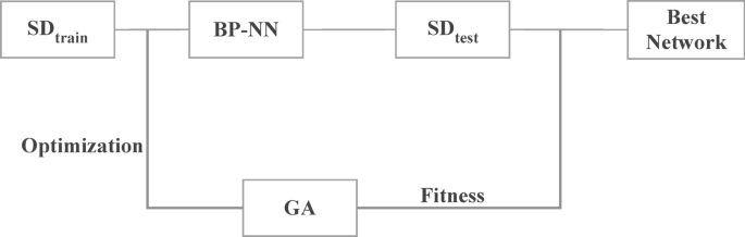
Structure of GA in student feature determination.


