Machine-learning-based reconstruction of Ming-dynasty defensive corridors in Yuxian

Research area

Given that Yuxian served as a key guard city under Xuanfu, which was one of the major strongholds of the Great Wall’s “Nine Frontier Defense Garrisons”, and considering its unique topographic structure and strategic pattern, this study focuses primarily on the natural geographical characteristics of Yuxian and their relationship with the defense system. The “Nine Frontier Defense Garrisons” refers to the frontier military system gradually established during the Hongwu to Jiajing periods of the Ming Dynasty, marked by the implementation of the Zongbing Regional Garrison System¹⁸.

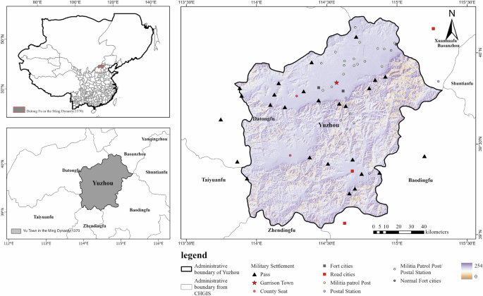
Yuxian in the Ming Dynasty was subordinate to Datong Prefecture(Datong Fu), governing three counties including Guangling, Lingqiu, and Guangchang. It is located in the northwestern part of Hebei Province, at the northwestern foot of the Taihang Mountains, and stands at the southernmost tip of Zhangjiakou. The geographical pattern Ming-dynasty Yuzhou comprised deep mountains in the south, river valleys in the middle, and hills in the north, with mountainous terrain surrounding it on all sides, naturally forming a lot of mountain passes and strategic passages. During the Ming Dynasty, in order to safeguard the capital and central plains, the central government constructed a defense system of inner and outer Great Walls west of Beijing. Yuxian occupied a critical buffer zone between these two walls and fell under the military jurisdiction of Xuanfu together with three neighboring towns, forming a mutually supportive strategic triangle. Key military garrisons such as Yuzhou guard city and Guangchang Defense Qianhu Suo (battalion) were established here, thus constructing the northern and southern defense lines of Yuzhou. Leveraging water systems, specifically the Huliu River, this county implemented an army farm strategy, making it a vital logistical supply base within the Great Wall defense system. This was also one of the reasons why Yuxian became the frequent target of raids by the northern pastoral nomads (Fig. 1).

Data sources

The data involved in this study can mainly be classified into the following categories:

Documentary Sources: Topographic data were sourced from the ASTER GDEM v2 digital elevation model (30 m resolution) provided by the Geospatial Data Cloud platform¹⁹. Following the clipping, filling and smoothing of the DEM, further raster derivatives such as slope, terrain undulation and Topographic Position Index (TPI) were generated. These metrics characterize natural conditions including mountainous resistance and gully-ridge structures, exerting constraints upon the layout of Yuxian’s peripheral zones and potential defensive corridors in the Ming Dynasty.

Historical Map Data: This study employed administrative division data from The Historical Atlas of China (Vol. 7), edited by Tan Qixiang²⁰, and the China Historical GIS (CHGIS) database from Harvard University²¹. The former provides a visual reference for the boundaries and military-administrative facilities of Yuxian around 1581, while the latter supplies the coordinates of administrative seats and their administrative affiliations during the Ming Dynasty.

The dataset of military sites is categorized into two subsets: research anchor data and model sample data. The research anchor data is derived from 65 heritage sites related to Yuxian as recorded in The Historical Atlas of China (THAC). Given the spatial positioning deviations inherent in historical maps, the precise coordinates of these sites were acquired through field surveys and UAV aerial photogrammetry. These coordinates were used for subsequent confidence assessment and study scope rectification, establishing a foundational point set for anchoring the research area. The model sample data was sourced from the China Great Wall Heritage Site²², which includes site locations of the Great Wall ramparts, watchtowers, horse-faces, and beacon towers. This dataset is utilized for subsequent defensive cost modeling and corridor inference.

Ancient transportation data were primarily drew from this research team’s prior systematic compilation of Yuxian’s historical postal relay and patrol dispatch systems. During the Ming Dynasty, the postal relay system fell under the jurisdiction of the Ministry of Rites and the Office of Communications, undertaking transportation and communication functions such as document delivery and reception of envoys. As non-military defensive nodes, relay stations and reconstructed post road networks were thus regarded as transportation nodes and passage frameworks, serving to construct road accessibility factors. In contrast, the patrol dispatch system operated within the military garrison system, primarily responsible for sentry duties and border outpost surveillance. Endowed with distinct military attributes for frontier containment and wartime support, patrol posts thus formed a military settlement system alongside guard cities, garrison towns, fortress settlements, and mountain passes. This system was employed to calculate defense core density, visual network indicators, and comprehensive defensive capability.

Historical Documents: Local gazetteers such as the Gazetteers of Yuxian County and the Gazetteers of Guangling County^23,24,25,26, along with their accompanying maps and other historical materials, were employed to verify the names, functions, and approximate locations of historical sites including guard cities, garrison towns, fortress settlements, mountain passes, and patrol posts. These findings were cross-referenced with the positions of surveyed archeological sites and historical base map data.

Research framework and technical route

The technical framework of this study comprises four interrelated stages, (Fig. 2). First, preliminary spatial analysis and input construction are conducted. Based on heritage site anchors, the validity of the historical study scope is verified. Elements such as spatial patterns, viewsheds, and the ancient post road network are preprocessed and quantified into indicators to generate basic raster variables. Accordingly, characteristic scales and spatial constraints are determined to provide a basis for subsequent stratified sampling and spatial cross-validation.

Subsequently, defense costs are defined, and machine learning modeling is performed. Based on cost factor screening and collinearity analysis, the defensive suitability variable is explicitly defined. A stratified sampling strategy combined with machine learning algorithms is then employed to train predictive models.

Following this, SHAP interpretability analysis is introduced to quantify the relative contribution of each factor and identify their directionality and non-linear effects on site distribution.

Finally, the construction of MCR defensive corridors is completed. Based on SHAP main effect curves, piecewise functions are constructed to map and normalize cost factor rasters via non-linear transformation, generating a new comprehensive resistance surface. Potential defensive corridors are then extracted based on this surface for further spatial interpretation.

Preliminary spatial analysis and input construction

Rationality verification of military defense settlement sites and historical boundaries

Prior to constructing the defensive cost model, we conducted a systematic confidence assessment of the heritage anchors to validate the rationality of the candidate study area. Based on Ming-dynasty frontier documents and historical maps of Yuxian, we geolocated and matched 65 site points within the unified spatial reference framework of THAC, and constructed an evidence-weighting index from three aspects—positional accuracy, chronological verifiability, and source reliability²⁷,as follows:

In Eq.(1), \({\mathrm{Conf}}_{i}\) denotes the point-wise confidence,\({C}_{p,i}\) represents position confidence; \({C}_{t,i}\) denotes chronological confidence; \({C}_{s,i}\) indicates source reliability. Each component is assigned according to a unified scoring sheet using a four-level ordinal scheme, and the weights are determined through expert elicitation.

In Eq.(2), \(N\) is the number of site points included in the assessment (this study:\(N\)=65).\({\mathrm{Conf}}_{\mathrm{overall}}\) is the arithmetic mean of the \({\mathrm{Conf}}_{i}\) values,which reflects the overall reliability of the military site dataset within the study area and supports the plausibility of the study-area delineation (Table S1).

Its comprehensive confidence is approximately 0.68. Based on this, a confidence-weighted site kernel density was generated (Fig. 3a) to explicitly address sample uncertainty arising from incomplete historical records (Table S2).

Because THAC does not provide county-level boundaries for the Ming dynasty, we compared the Datong Prefecture boundaries across the time slices available in THAC. Relative to 1369, the 1371 prefectural boundary shows a pronounced southeastward expansion, and this spatial configuration remains broadly stable through the Wanli period. In light of historical records on Yuzhou’s administrative reassignment to Datong Prefecture in the early Hongwu reign²⁸, this increment corresponds closely to the documented adjustment in Yuzhou’s administrative affiliation. We therefore treat the incremental area of the 1371 prefectural boundary relative to 1369 as a proxy for the early-Ming administrative extent of Yuzhou, rather than as county-boundary ground truth.

We then assessed the plausibility of this proxy extent using three quantitative indicators (Table 1): terrain conformity, edge-settlement distance to the boundary, and boundary coverage. The proxy extent performs consistently well across these indicators. Moreover, when overlaid with the present-day administrative boundaries of Yuxian and its three neighboring counties (Guangling, Lingqiu, and Laiyuan), it shows strong overall agreement in macro-scale form (IoU ≈ 0.92; Fig. 3b). High-overlap segments between the proxy and modern boundaries are concentrated along high-elevation ridgelines and watershed divides (Fig. 3c). In addition, more than 90% of high-confidence defensive settlements fall within the intermontane basins and Great Wall–pass corridors enclosed by the proxy extent, suggesting that the study area is jointly shaped by persistent topographic structure and the defensive system. Accordingly, we adopt the 1371-derived proxy extent as the analytical study area, and within a 1-km buffer of this boundary we screen 278 defensive heritage sites as positive samples for subsequent modeling (Fig. 3d).

Spatial pattern Analysis

Compared with the independent dataset of heritage anchors previously used to define the study scope, this study further selected 278 field-surveyed military sites within the study area for spatial pattern analysis (Table 2). First, kernel density estimation was applied to smooth the point sites into a continuous defensive intensity raster, yielding the spatial intensity distribution of military defense facilities in the study area(Fig. 3d). The formula is as follows:

In Eq.(3), \(\hat{f}(s)\) denotes the estimated probability density at location\(s\); \(n\) is the number of sample point; \(h\) is the bandwidth;and\({s}_{i}\) is the coordinate of the \(i\)-th sample point. Second, the average nearest neighbor distance of the point-like pattern was calculated under Euclidean distance measurement using the site elements as input. Based on the Complete Spatial Randomness (CSR) assumption, the theoretical expected distance and Nearest Neighbor Ratio (R) were derived, and the Z-score and p-value were used to test whether it significantly deviates from a random distribution.The formula is as follows:

In Eq.(4), \({\bar{d}}_{o}\) is the observed mean nearest-neighbor distance, \({\bar{d}}_{e}\) is the expected mean distance under complete spatial randomness (Poisson),\(A\) is the study area and n is the number of points. \(R\)>1 indicates dispersion and \({R}\)<1 indicates clustering.

Finally, the Moran’s I index of military settlements was calculated under inverse distance weighting and Euclidean distance adjacency to test their spatial autocorrelation.

The formula is as follows:

In Eq.(5),n denotes the number of military defense settlement sites,\({x}_{i}\) is the kernel density (or settlement density) value associated with site\(i\). \(I\) > 0 indicates clustered military settlements,\(I\) < 0 indicates dispersed settlements.

In subsequent model construction, these high-density areas were used as candidate regions for potential defense corridors, serving to construct settlement density costs and assist in determining the stratified sampling scope.

Construction of visual network and extraction of visual distance control factors

The military defense system of the Ming Dynasty exhibited distinct linear visual control characteristics. Particularly along the Great Wall and border defense lines, a beacon tower system and military settlements formed an information transmission network relying on visual distance connectivity, aiming to enable timely defensive responses to early warning messages. To quantitatively evaluate the spatial control capability of Yuxian in the Ming Dynasty, this study constructed a regional viewshed network using cumulative viewshed analysis and linear intervisibility analysis. Observation and target height offsets were set according to the different structural heights of military settlement facilities: a uniform 1-m eye-level height was added as the observation offset for simulating observers, while an 8-m smoke height was added as the target offset for simulating observed objects¹³. For any observed beacon tower site, the offset was the sum of its own facility height and the smoke height (Table 3). Some sites along the Great Wall showed low visibility frequencies in the cumulative viewshed. However, they were actually connected by walls and possessed visual connectivity. Therefore, the wall connection relationship was approximately introduced to assist in judging the viewshed connectivity of such facilities.

Complex Network Analysis (CNA) identifies the importance of military settlements in the visual network by indexing the intervisibility relationships between nodes. This study selected indicators including node degree, betweenness centrality, and closeness centrality^29,30,31 (Table 4), to evaluate three key aspects: the settlements’ visual distance connectivity capability within local areas, their significance as relay hubs in the overall network, and their average path length to all other visible nodes, reflecting their control efficiency and information response speed in the global structure. Meanwhile, network density and visual inclusiveness were used to assess the integrity and node coverage rate of the global visual network (Fig. 4). Indicators such as Intvis_den and Betweenness, constructed based on cumulative viewshed and intervisibility network, collectively show (Fig. 4 and Table 5) that the visual network possesses certain connectivity and node heterogeneity. This provides a structural foundation for subsequent extraction of defensive cost factors including visual line density and node centrality (Fig. 5).

Reconstruction of ancient post road network and construction of transportation cost factors

The transportation corridors of the Ming Dynasty played a crucial role in troop deployment and material transportation within the military defense system, with their passability and accessibility regarded as core constraints for road selection. First, this study identified transportation nodes such as post stations and mountain passes based on records of the postal relay and patrol dispatch systems in ancient documents. Combined with the county territory maps attached to local gazetteers (Fig. 6), the study spatially registered each symbol of the postal relay and patrol dispatch systems as well as military settlement on the maps one by one. Furthermore, according to the node accessibility relationships indicated by the post route lines on the maps, preliminary connection paths were drawn between adjacent transportation nodes, serving as a prior guide for directions and corridors. Finally, drawing on the research methods for post road reconstruction in the Datong Prefecture proposed by Yingchun Cao et al.³², a transportation cost surface was constructed with core factors including slope, terrain undulation, and river crossing cost. On this basis, the Least Cost Path (LCP) method was used to connect various nodes to generate the ancient post road network within Yuxian. The reconstructed ancient post road network was used not only to construct the cost factor of the distance to ancient post road, but also to provide a comparative benchmark for judging the coupling relationship between defense corridors and the existing transportation network.

Construction of the defensive cost model

The defensive cost model constructed in this study is essentially a predictive framework based on environmental features, designed to quantify the locational preferences of Ming Dynasty military facilities using machine learning algorithms.The model designates spatial “defensive suitability” as the target variable. Based on the foundational raster variables obtained from the preceding analysis and multi-source data, a system of three cost factor categories was constructed. Subsequently, a stratified sampling strategy was implemented to generate a negative sample set equal in size to the positive samples. Logistic Regression (LR), Random Forest (RF), and XGBoost models were then employed to derive (or predict) suitability probabilities. Given the intrinsic robustness of the selected ensemble tree models to feature scaling, data normalization was not applied globally during the machine learning phase. Instead, standardization was applied exclusively to the input features for the LR model. Global feature normalization was deferred to the subsequent stage of constructing the SHAP-based resistance surface.

Selection of cost factors

During the Ming Dynasty, the beacon tower system in Yuxian was interconnected relying on terrain, forming a hierarchically distinct early warning network. Meanwhile, the transportation system connected various nodes in series through post roads, constituting the basic traffic framework. Correspondingly, for military key points such as guard cities, garrison towns, and mountain passes that undertook strategic maneuver and defensive deployment, the construction of the defense corridors behind them also followed specific spatial preferences and selection logic.

The quantification of defensive capabilities of military defense sites and landscape nodes helps explain their relative importance¹³, as well as the spatial logic underlying the formation of defense corridors. Existing archeological site prediction models³³ mainly analyze the relationship between geographical factors and the spatial distribution of sites to predict the probability of sites appearing in specific spatial areas. In such models, topographic and environmental characteristics are usually regarded as potential cost factors closely related to defensiveness^34,35. Based on this, settlement density, cumulative viewshed, visual line density, and node centrality were selected as defensive cost factors to reflect the defensive performance of sites in terms of information transmission, viewshed control, and spatial connectivity. Meanwhile, indices such as elevation, slope, TPI, TRI, and surface relief were chosen as geographical cost factors, and distance to post roads, distance to the Great Wall, distance to defensive nodes, and distance to water sources as distance cost factors. Together, these constitute the candidate cost system for the subsequent defensiveness model (Table 6).

Screening of correlation and multicollinearity among cost factors

Prior to conducting defensive cost modeling based on machine learning, to ensure the consistency of various raster factors in terms of spatial location and resolution, unified spatial preprocessing was performed on all raster data: All data were projected to the WGS_1984_UTM_Zone_50N coordinate system, with the 30 m resolution DEM used as the Snap Raster. Bilinear interpolation was adopted for resampling continuous variables, while the Inverse Distance Weighting method was used to supplement a small number of missing values in node centrality indicators and generate continuous raster surfaces. For distance cost factors, Euclidean distance rasters were used as continuous variable inputs to avoid subjectivity caused by classification thresholds and loss of rank information. The above-mentioned processing provided a consistent-scale raster data foundation for subsequent correlation analysis and cost factor screening.

On the basis, it is necessary to test and control the correlation and multi collinearity among various cost factors. Existing studies have shown that high correlation among environmental factors will increase the risk of model overfitting, weaken the physical meaning of the interpretation of variable importance, and thus make the model more likely to fit noise rather than true patterns^36,37. To eliminate potential multicollinearity among candidate cost factors, this study first adopted Spearman’s rank correlation coefficient to analyze the monotonic correlation between variables, and subjected highly correlated factors to preliminary elimination. Subsequently, the Variance Inflation Factor (VIF) was calculated to identify sources of redundancy and perform iterative elimination, so that the multicollinearity among the retained variables was controlled within an acceptable range (VIF < 5)³⁸. This ensures the stability and interpretability of the modeling process.

Spearman’s rank correlation analysis shows (Fig. 7) that the absolute values of correlation coefficients between most cost factors are less than 0.5, indicating a relatively low overall correlation level. An extremely strong positive correlation is only observed between Slope and the TRI (ρ = 0.94). In addition, there exist moderate positive correlations between the kernel density of military settlements (KD_military) and node betweenness centrality (Betweenness), between KD_military and visual line density (Intvis_den), as well as between Betweenness and Intvis_den (|ρ | = 0.48–0.62). However, none of these correlations exceed the empirical threshold of 0.8³⁹. Subsequently, the calculated results of Variance Inflation Factor (VIF) are presented in Table 7. The VIF values of DEM, Slope, and TRI are 12.51, 15.96, and 14.68 respectively, which are significantly higher than 10, indicating severe linear overlap among the three factors. The VIF values of all other variables range from 1.72 to 4.84, reflecting a generally low level of multicollinearity. Combined with the correlation coefficient matrix, it can be concluded that the excessively high VIF values are mainly caused by the redundancy of slope-related indicators.

Referring to the processing principle of eliminating variables with |ρ | >0.8 in previous studies, as well as the physical meaning and interpretability of indicators, this study retained Slope (representing the first-order slope gradient) and Rugged (indicating the terrain ruggedness), while eliminating TRI, which is highly redundant and most strongly correlated with Slope. Subsequently, a repeated correlation check showed that the absolute correlation coefficients among the remaining 12 cost factors were all below 0.6. Regarding the VIF results, all variables had VIF values below 5 except for DEM (12.51). Considering that DEM has an independent and critical physical significance in geomorphological processes, and the subsequent main ensemble learning models such as RF and XGBoost are insensitive to linear multicollinearity between variables, DEM was retained. On the other hand, since most military defense facilities were built adjacent to the Great Wall, including the “distance to the Great Wall” in the model would easily excessively overstate its explanatory power, thereby obscuring the true contributions of other cost factors. Thus, this variable was eliminated. Finally, a total of 11 cost factors were selected for modeling.

Stratified sampling strategy

This study used 278 verified measured site points, which were screened based on previously validated boundaries, as positive samples, and adopted a lightweight stratified sampling strategy constrained by the Great Wall survey lines. First, the Great Wall section from Langya Pass to Wulong Castle, as well as military settlements such as mountain passes and forts along this section, were selected to construct a linear constraint zone of defensive settlements with defensive attributes. This defensive settlement zone has been depicted as an important defensive belt in the southern part of the county in various ancient maps and documents^40,41,42. Subsequently, Near analysis (Near) was used to calculate the shortest distance from each site point to the Great Wall survey lines, and their distribution characteristics across different distance gradients were counted. On this basis, five distance belts (2 km, 5 km, 10 km, 20 km, and 40 km) were set. Within each distance belt, background points were randomly selected as negative samples at a 1:1 ratio relative to the number of positive samples (Table 8). To avoid spatial overlap and category interference in geographical locations, the selection of negative samples was subject to the condition that they did not coincide with site points within a 300 m circular buffer zone. This stratified sampling strategy ensures that positive and negative samples have comparable environmental conditions near the Great Wall buffer zone, thereby improving the model’s ability to distinguish subtle differences in the site selection preferences of historical settlements.

Machine learning modeling

This spatial pattern analysis in the previous section (Table 2) indicated that military defense sites exhibit a significantly clustered distribution (Mean Nearest Neighbor Ratio R = 0.42, z = –18.53, p < 0.001), and the defensive intensity field shows strong spatial positive autocorrelation (Moran’s I = 0.967, z = 15.96, p < 0.001). If traditional random cross-validation is adopted, it will lead to a high degree of interdependence between the training set and the test set at the 1–3 km scale, thereby underestimating the generalization error. To mitigate the impact of spatial autocorrelation, this study employed spatial block cross-validation: Regular grids with a side length of approximately 7 km were generated within the study area, dividing it into 154 spatial blocks. These blocks were further partitioned into 5 folds, with each fold containing a set of spatially relatively continuous grids and approximately 20% of the sample points. During model training, 4 folds were alternately used as the training set, and the remaining 1 fold as the test set. This ensures that the typical spatial interval between the test set and the training set is greater than approximately 3 km, which exceeds the main distance scale of the aforementioned spatial autocorrelation effect. To compare the bias effect of traditional methods, a control group with 5-fold random cross-validation (CV) was also established (Fig. 8). To reduce fluctuations caused by random partitioning and improve the reproducibility of results, a fixed random number seed (42) was used for initialization when constructing cross-validation and training models involving random processes (such as RF and XGBoost).

Within the framework of spatial block cross-validation, three models including RF, LR, and XGBoost were selected to invert and calculate the influence weights of each cost factor. The LR model can explain the directionality and linear weights of each cost variable, while the RF and XGBoost models use the results of the LR model as a linear baseline to further reveal the nonlinear influence preferences of each cost variable and their importance ranking. Based on the 556 sample points obtained from the aforementioned stratified sampling strategy, a binary response variable for modeling was first constructed. The dependent variable was defined as ‘defensive locational suitability’, assigning a value of 1 to positive samples and 0 to negative samples, thereby obtaining a label variable y taking values in {0,1} to distinguish between the positive and negative sample sets.

Furthermore, a grid search was conducted to optimize the hyperparameter combinations for each model. Specifically, for the LR model, input features were pre-standardized to ensure the convergence speed of gradient descent and the effectiveness of regularization. The model was configured using L2 regularization (penalty = ‘l2’) and the ‘liblinear’ solver. The optimal value of the regularization parameter C was determined via cross-validation within the range of {0.01, 0.1, 1, 10} to prevent model overfitting. The LR model formula is as follows:

In Eq (6),\({p}_{i}\) represents the predicted probability of site/settlement occurrence for sample \(i\), given the vector of cost factors \({x}_{i}\).

For the RF model, the number of decision trees was set to the range {100, 200, 300} to control the scale of the forest; the maximum depth was set to {5, 7, None}, where “None” indicates no restriction on tree depth, serving to adjust the complexity of individual trees; the minimum number of samples per leaf node was set to {1, 3} to limit the minimum sample size contained in leaf nodes, thereby achieving regularization and smoothing of predictions. A subset of features was randomly selected at each node for splitting to enhance the diversity among individual trees and reduce the risk of overfitting. For the XGBoost model, the learning rate (learning_rate) was set to {0.01, 0.05, 0.1} to control the update step size of each tree on the overall model; the max_depth was set to {3, 5, 7}, with shallow trees helping avoid over-splitting when the sample size is limited, while deep trees are used to characterize complex nonlinear relationships; the number of trees (n_estimators) was set to {100, 200, 300}, corresponding to a medium-scale ensemble of trees; the subsample ratio (subsample) was set to {0.8, 1.0}, which not only ensures sample utilization efficiency but also introduces a certain degree of regularization through random subsampling of samples. Other regularization-related hyperparameters, such as the column sampling ratio (colsample_bytree), the minimum sum of instance weights needed in a child (min_child_weight), and the L2 regularization term coefficient (reg_lambda), adopted the default settings of XGBoost to avoid excessive expansion of the parameter space. Finally, AUC (Area Under the ROC Curve), PR-AUC (Area Under the Precision-Recall Curve), and Brier score were used to comprehensively evaluate model performance. AUC measures the overall ability to distinguish between positive and negative samples; PR-AUC focuses more on the recognition performance for positive classes (sites); the Brier score characterizes the consistency between predicted probabilities and actual observations. In general, AUC and PR-AUC values higher than 0.8 and close to 0.9 or above are considered to indicate good discrimination performance, while a Brier score significantly lower than approximately 0.25 (the baseline value for random predictions) indicates high probability prediction performance. The Brier score formula is as follows:

In Eq.(7), \({{\rm{p}}}_{{\rm{i}}}\) is the predicted probability of site occurrence output by the model, and \({{\rm{y}}}_{{\rm{i}}}\) is the observed label (0/1).

SHAP interpretability analysis

To further explain the site selection patterns of military defense settlements learned by the machine learning model and quantify the relative contributions of each cost factor to the probability of site occurrence, SHAP was introduced for interpretability analysis based on the selected optimal model⁴³. SHAP is based on the game-theory-derived Shapley value principle⁴⁴, which regards the model output as the result of collaborative contributions from various features. By comparing the predictive changes of the model before and after adding or removing a specific feature, the direction and magnitude of the marginal contribution of that feature to the prediction of individual samples are calculated. For each sample-feature combination, a positive SHAP value indicates that the corresponding cost factor will increase the predicted probability of a defensive settlement appearing at that location, while a negative value indicates an inhibitory effect. The absolute value reflects the intensity of the influence. The formula is as follows:

In Eq.(8), \(N\) denotes the entire set of features, \(S\) represents the subset excluding feature \({\rm{i}}\), and \({\rm{f}}({{\rm{x}}}_{{\rm{S}}})\) denotes the model output when only the feature subset \({\rm{S}}\) is used.

On the global scale, averaging the SHAP values of each cost factor yields a set of model structure-independent feature importance rankings. This ranking is used to measure the relative weights of each cost factor in explaining the spatial distribution of defensive settlements, complementing the linear weights derived from LR coefficients. On the local scale, SHAP scatter plots and dependence plots are employed to examine the nonlinear responses of predicted probabilities to changes in the values of individual factors, thereby identifying key threshold intervals. Examples include “the optimal distance range from the Great Wall for fortress construction” and “the threshold intervals for slope and viewshed conditions”. This method can convert the implicit site selection preferences embedded in black-box models into interpretable spatial rules, providing a basis for subsequent defensive suitability mapping and defense corridor extraction⁴⁵.

Defense corridor modeling based on MCR

To quantify the preference effect of defensive cost factors on potential defense corridors, this study constructed non-linear resistance functions based on SHAP main effect curves. Through continuous reclassification, the suitability contribution of each factor was transformed into resistance values. Subsequently, a comprehensive resistance surface was generated via weighted summation, and the MCR model was employed to identify the defense corridors. First, spline smoothing was applied to SHAP main effect curves and pairwise relationship plots to obtain continuous main effect functions \({g}_{k}({z}_{k})\). For factors showing an overall monotonic trend within their value ranges, the sign and slope of \({g}_{k}\) were directly used as the basis for the direction and magnitude of cost changes with factors. For factors with a unimodal or U-shaped trend, the curves were divided into several local monotonic intervals at the global extreme values. Within each interval, piecewise linear approximation was performed using endpoint connection lines, thereby obtaining the continuous approximate main effect \({\widetilde{C}}_{k}({z}_{k})\). Subsequently, one-dimensional linear interpolation was conducted on the factor values of each pixel, followed by linear normalization within the range of the 5th to 95th percentiles. The results were then truncated to the [0,1] interval to generate standardized single-factor resistance rasters. The formula is as follows:

In Eq.(9), \(x\) denotes a raster cell, \({C}_{k}(x)\) represents the normalized single-factor cost raster, \({w}_{k}\) is the corresponding weight, and \(k\) is the number of cost factors involved in the superposition. Equal weight setting is uniformly adopted for each cost factor, i.e., \({w}_{k}\) = 1/K. SHAP values are not directly used as the source of weights.

To identify potential defense corridors, this study took military settlements and mountain passes with defensive attributes as source points, and calculated the MCR surface using cost-distance analysis on the comprehensive defense cost surface. Subsequently, equal-area and natural breaks classification was performed on the cumulative resistance values, and several levels with the lowest resistance were extracted as potential corridor zones with the highest defensive suitability. These zones were further simplified into a continuous defense corridor network through skeleton extraction and raster-to-line conversion. On this basis, to test the sensitivity of the predicted defense corridors to cost factor configuration and topographic data resolution, two sets of robustness experiments were designed: (1) With other settings unchanged, three types of key factors including visual line density, slope, and kernel density of military settlements, were removed respectively to reconstruct the comprehensive cost surface and corridor network; (2) The modeling process was repeated using 90 m resolution DEM to obtain resolution-controlled corridors. By comparing indicators such as the overlap ratio within the 1 km buffer zone, total length change, line position offset, and shape overlap degree under the 1 km buffer zone between each scenario and the 30 m DEM baseline corridor, the two sets of experiments evaluated the robustness of the model of parameter setting.