Now we'll use voting, bagging, and random forests to ensemble learning.
Voting itself is just a counting mechanism. No diversity is created, but predictions from already different models are combined.
Bagging, on the other hand, explicitly creates diversity by training the same base model on multiple bootstrap versions of the training dataset.
Random forests extend bagging by further restricting the set of features considered in each split.
From a statistical perspective, the idea is simple and intuitive. Randomness creates diversity without introducing fundamentally new modeling concepts.
But ensemble learning is much more than that.
does not rely on randomness at all, optimization. Gradient boosting belongs to this family. To really understand it, start with an intentionally weird idea.
Apply gradient boosting to linear regression.
yes i know. This is probably the first time you've heard of applying gradient-boosted linear regression.
(Tomorrow we will discuss gradient boosted decision trees).
In this article, we plan to:
- First, let's take a step back and revisit the three basic steps of machine learning.
- Next, we introduce the Gradient Boosting algorithm.
- Next, apply Gradient Boosting to your linear regression.
- Finally, let's consider the relationship between Gradient Boosting and Gradient Descent.
1. Machine learning in three steps
To make machine learning easier to learn, I always break it down into three distinct steps. Let's apply this framework to gradient-boosted linear regression.
Because unlike bagging, each step reveals something interesting.

1. Model
A model is something that takes input features and produces output predictions.
The base model in this article is linear regression.
1 screw. ensemble method model
Gradient boosting is do not have The model itself. This is an ensemble method that aggregates multiple base models into a single metamodel. By itself, it does not map inputs to outputs. Must be applied to the base model.
Here we use gradient boosting to aggregate a linear regression model.
2. Model fitting
Each base model must be fit to the training data.
For linear regression, fitting means estimating the coefficients. This can be done numerically using gradient descent, but it can also be done analytically. In Google Sheets or Excel, LINEST A function that estimates these coefficients.
2 screws. Ensemble model learning
At first, Gradient Boosting may seem like a collection of simple models. But it's still a learning process. As we will see, it relies on a loss function, just like the classical model that learns weights.
3. Model tuning
Model tuning consists of hyperparameter optimization.
In our case, the base model linear regression itself has no hyperparameters (unless we use regularized variants such as Ridge or Lasso).
However, gradient boosting introduces two important hyperparameters: the number of boosting steps and the learning rate. This will be explained in the next section.
In short, machine learning can be done in three easy steps.
2. Gradient boosting regression algorithm
2.1 Algorithm principle
Here we present the main steps of the gradient boosting algorithm applied to regression.
- Initialization: We start with a very simple model. For regression, this is usually the mean value of the target variable.
- Calculating residual error: Computes the residual, defined as the difference between the actual value and the current prediction.
- Fit linear regression to residuals: Fit a new base model (here a linear regression) to these residuals.
- Update the ensemble : Add this new model to the ensemble and scale it by the learning rate (also known as shrinkage).
- repeat the process: Repeat steps 2-4 until the desired number of boosting iterations is reached or the error converges.
that's it! This is the basic procedure for performing gradient boosting applied to linear regression.
2.2 Expressing the algorithm as a formula
You can now write formulas explicitly, which helps make each step more specific.
Step 1 – Initialization
Start with a constant model equal to the mean of the target variable.
f0 = average(y)
Step 2 – Calculate residuals
Compute the residual, defined as the difference between the actual value and the current prediction.
r1 = y − f0
Step 3 – Fit the base model to the residuals
Fit a linear regression model to these residuals.
r̂1 = a0 · x + b0
Step 4 – Update the ensemble
Update the model by adding the fitted regression scaled by the learning rate.
f1 = f0 − learning rate · (a0 · x + b0)
next iteration
Repeat the same steps.
r2 = y − f1
r^2 = a1・x + b1
f2 = f1 − learning rate · (a1 · x + b1)
Expanding this formula, we get:
f2 = f0 − learning rate・(a0・x + b0) − learning rate・(a1・x + b1)
The same process continues with each iteration. The residuals are recalculated, a new model is fitted, and the ensemble is updated by adding the learning rate to this model.
This formulation makes it clear that Gradient Boosting builds the final model as the sum of successive correction models.
3. Gradient-boosted linear regression
3.1 Training the basic model
I'll start with a simple linear regression as the basic model, using a small dataset of 10 observations that I generated.
For basic model fitting, use the Google Sheet function LINEST to estimate linear regression coefficients (also works in Excel).

3.2 Gradient boosting algorithm
These formulas are easy to implement in Google Sheets or Excel.
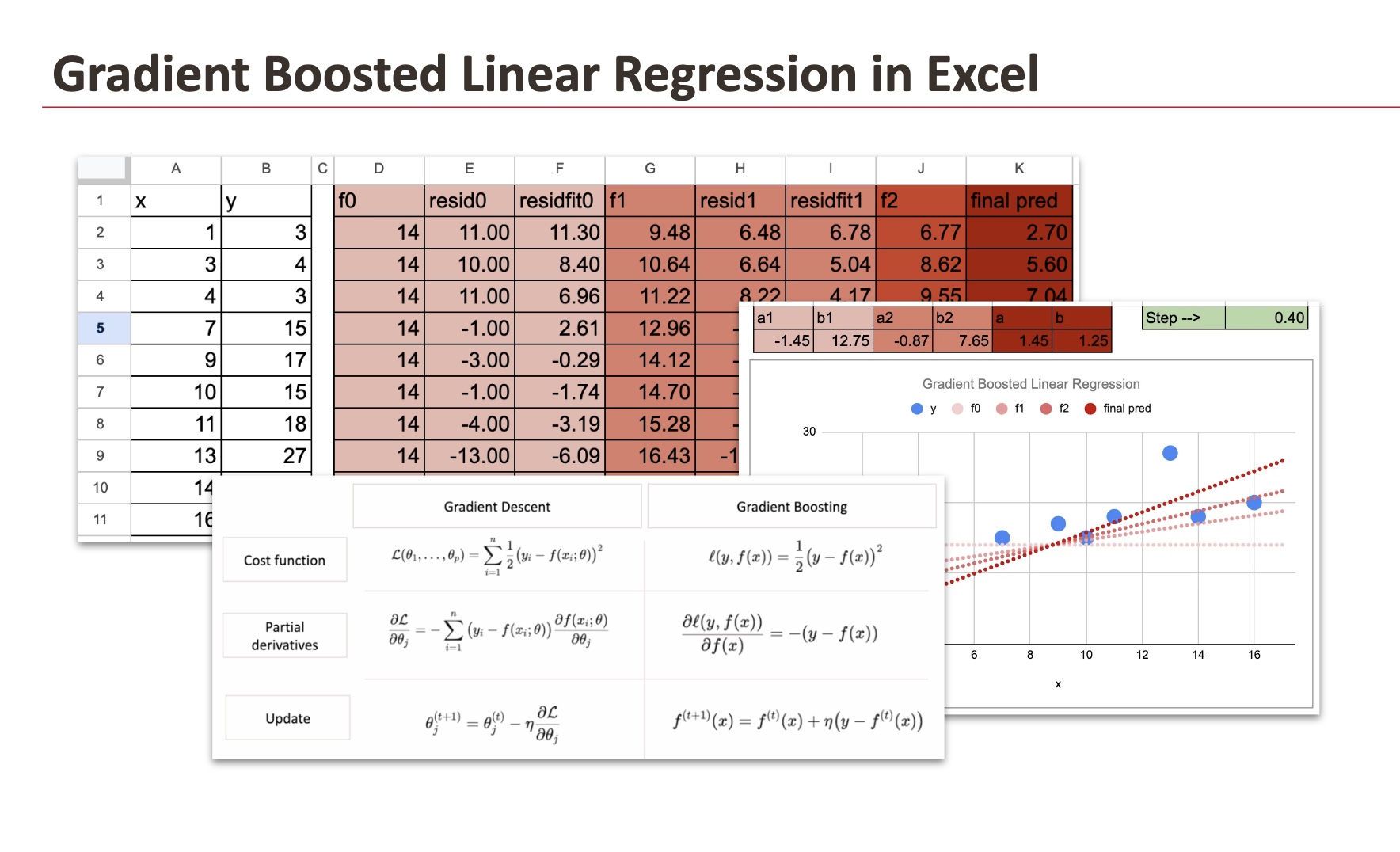
The table below shows the training dataset and the various steps in the gradient boosting step.

Each fitting step uses the Excel function LINEST.

We only do two iterations, but you can guess what happens with more iterations. Below is a diagram showing the model at each iteration. The various shades of red indicate the convergence of the model, as well as the final model found directly with gradient descent applied directly to y.

3.3 Why boosting linear regression is purely educational
A careful look at the algorithm yields two important observations.
First, in step 2, we fit a linear regression to the residuals. The model fitting step takes time and algorithmic steps to accomplish. Instead of fitting a linear regression to the residuals, we can fit a linear regression directly to the actual values of y and the final best-fit model has already been found.
Then if you add a linear regression to another linear regression, it's still a linear regression.
For example, f2 can be rewritten as:
f2 = f0 – learning rate * (b0+b1) – learning rate * (a0+a1) x
This is still a linear function of x.
This explains why gradient-boosted linear regression provides no practical benefit. Its value is purely educational. It helps you understand how gradient boosting algorithms work, but it does not improve predictive performance.
In fact, this is even less useful than bagging applied to linear regression. Bagging allows you to estimate prediction uncertainty and construct confidence intervals due to the variation between bootstrap models. Gradient-boosted linear regression, on the other hand, reverts to a single linear model and provides no additional information about uncertainty.
As we'll see tomorrow, the situation is very different when the underlying model is a decision tree.
3.4 Adjusting hyperparameters
There are two hyperparameters you can tune: number of iterations and learning rate.
Although we have only implemented two iterations, it is easy to imagine more iterations, which can be completed by examining the magnitude of the residuals.
As for the learning rate, you can change it in Google Sheets and see what happens. A small learning rate slows down the “learning process”. If the learning rate is 1, you can see that it converges in iteration 1.

And the residual for iteration 1 is already zero.

If the learning rate is higher than 1, the model diverges.

4. Boosting as gradient descent in function space
4.1 Comparison with gradient descent algorithm
At first glance, the role of learning rate and number of iterations in gradient boosting is very similar to that seen in gradient descent. This naturally causes confusion.
- For beginners You often notice that both algorithms contain the word “.gradientSo it's tempting to assume that gradient descent and gradient boosting are closely related, without actually knowing why.
- experienced practitioner They usually react differently. From their perspective, the two methods appear unrelated. Gradient descent is used to fit weight-based models by optimizing parameters, while gradient boosting is an ensemble technique that combines multiple models with fitted residuals. The use cases, implementations, and intuitions look completely different.
- at a deeper levelHowever, experts will tell you that these two algorithms are actually the same optimization idea. The difference lies not in the learning rules, but in the space in which these rules are applied. Alternatively, you could say that the variables of interest are different.
Gradient descent performs gradient-based updates. parameter space. Gradient boosting performs gradient-based updates. function space.
That's the only difference in this mathematical numerical optimization. Let's look at the equations for the regression case and the general case below.
4.2 For mean squared error: same algorithm, different space
Using mean squared error, gradient descent and gradient boosting minimize the same objective and are driven by the same amount: the residual.
In gradient descent, residuals influence updates of model parameters.
In gradient boosting, the residuals directly update the prediction function.
In both cases, learning rate and number of iterations play the same role. The difference lies only in where the updates are applied: parameter space and function space.
Once this distinction becomes clear, it becomes clear that gradient boosting using MSE is simply gradient descent expressed at the level of functions.

4.3 Gradient Boosting with Arbitrary Loss Function
The above comparison is not limited to mean squared error. Both gradient descent and gradient boosting can be defined in terms of different loss functions.
In gradient descent, loss is defined in parameter space. This requires that the model be differentiable with respect to the parameters, which necessarily limits the method to weight-based models.
In gradient boosting, the loss is defined in the prediction space. Only the loss must be differentiable with respect to the prediction. The base model itself does not need to be differentiable, and certainly does not need to have its own loss function.
This explains why Gradient Boosting can combine arbitrary loss functions with non-weight-based models such as decision trees.

conclusion
Gradient boosting is not just a simple ensemble method; it is an optimization algorithm. It follows the same learning logic as gradient descent, only the space (parameters and functions) in which the optimization is performed differs. Using linear regression, we were able to isolate this mechanism in its simplest form.
In the next article, we'll see how this framework becomes truly powerful when the base model is a decision tree, leading to gradient-boosted decision tree regressors.
All Excel files are available at this Kofi link. Your support means so much to me. Early supporters get the best deal as the price increases mid-month.