Land use classification plays an important role in agriculture, urban planning, and environmental monitoring. The work focus on developing a new ensemble network based on deep learning (i.e., InceptionResNet-UNet architecture) for land use classification of historical Sentinel-2 images.
The proposed workflow includes three major stages:
-
1.
Data collection and preprocessing
-
2.
Model architecture design
-
3.
Training, validation, and evaluation
Data collection and preprocessing
Source: Sentinel-2A and Sentinel-2B imagery (10m spatial resolution) were downloaded via NRSC-Bhuvan44 and Google Earth Engine45.
Tool used to process : QGIS version 3.22 (https://qgis.org).
Study area: Katpadi region, Vellore district, Tamil Nadu, India.
Time Span: 2017–2024 (images from peak season: March–May).
Classes: 8 major land use categories.
Preprocessing steps:
-
Atmospheric correction using Sen2Cor
-
Image tiling into 256 × 256 pixel patches
-
Manual annotation using QGIS and validation through field surveys
-
Georeferencing and projection standardization (UTM Zone 44N)
For this work, we acquired multi-year Sentinel-2 images of the Katpadi area of Vellore District (Tamil Nadu), which is located in a strategically important region linking three states (Tamil Nadu, Andhra Pradesh and Karnataka) as shown in Fig. 1. The map has been with national and state routes passing through Vellore, it features an archetypal geographical chart of wildlife sanctuaries, mountains, bursting rivers, and many bright lakes. Katpadi, among other towns, shows a population boom as a result of unplanned urban growth. For this reason, the region is ideal for tracking long-term land-use changes. Figure 1 was an open access data developed by district survey office, Vellore and was published in Vellore Institute of Technology website.

Source Vellore Institute of Technology—https://vit.ac.in. Data Source : NRSC Bhuvan portal— and processed using QGIS 3.22.
We did land use monitoring and change detection using historical Sentinel-2 images from NRSC-Bhuvan portal (https://bhuvan.nrsc.gov.in) and Google Earth. Images underwent rigorous preprocessing steps, namely radiometric calibration, atmospheric correction and cloud masking, to ensure sufficiently high data quality for analysis. The tools used to process these images is QGIS version 3.22 (https://qgis.org). A representative of the model-training dataset is shown in Fig. 2. We have categorized the dataset into different classes like forests, rivers, building, water bodies, trees etc.

Sample Dataset used to train the model. Data Source: NRSC Bhuvan portal—https://bhuvan.nrsc.gov.in and processed using QGIS 3.22.
Data preparation
We divided the acquired dataset into training, testing, and validation subsets. We normalized the image pixel values to a standard range (e.g., 0–1) to ensure consistency in data representation. This step is necessary to properly train the model proved to be effective.
To address the challenging satellite image segmentation task, IRv2-Net is a hybrid model architecture which combines an InceptionResNetV2 and UNet backbone. InceptionResNetV2: We selected InceptionResNetV2 since it is well regarded in the literature as a successful photo-based feature extractor, especially on multi-scale features. This is due to its combination of various kernel size-based convolutions, which effectively preserve both fine and coarse features in satellite data.
Through the use of skip connections that help restore spatial context lost in the downstream encoding stage, the UNet integrated design makes segmentation work well. Fusion techniques strike a balance between detailed feature extraction and pixel-wise segmentation and are therefore also suitable for complex classification tasks like satellite image classification. In this study, we propose such quality classification of land covers types by using an IRU-Net (Input-residual update-based neural network) all capable of extracting the spatio-temporal dynamics of the processes involved with land use and land cover change leading to improved efficiency with respective classification of land cover types of interest over the Katpadi region.
Normalization of Pixel Values (Eq. 1): To represent data consistently, normalize pixel values to fall between 0 and 1.
$${\text{I}}\_{\text{norm}} = \left( {{\text{I}} – {\text{I}}\_{\text{min}}} \right)/\left( {{\text{I}}\_{\text{max}} – {\text{I}}\_{\text{min}}} \right)$$
(1)
where I is the pixel value, I_min and I_max are the minimum and maximum pixel values in the dataset, respectively.
IRUNet architecture
The architecture consists of:
-
Encoder InceptionResNetV2 pretrained on ImageNet. Decoder: UNet-style upsampling layers.
-
Skip connections Between encoder and decoder blocks.
-
Fusion Multi-level feature fusion at bottleneck.
-
Test-time augmentation Horizontal and vertical flipping during inference to enhance robustness.
The IRUNet architecture takes in 256 × 256 × 3 images as input, and the pre-trained ImageNet weights are used to set up the convolutional filters in InceptionResNetV2. The encoder, bridge, and decoder comprise the three main components of the UNet architecture. We implemented the encoder in a standard UNet style, with 4 downsampling blocks, each made from two convolutional layers and one max-pooling layer. A filter size of 3 × 3 is used for the convolutional layers while a filter size of 2 × 2 is adopted for the max-pooling layers, which progressively reduces spatial dimensions and increases the depth of feature maps.
Feature extraction
In the IRUNet, the Inception ResNet-v2 blocks replace these conventional encoder blocks. Each Inception block is followed by a filter expansion layer (1 × 1 convolution without activation) to adjust the depth of the filters. The architecture extracts intermediate activations from the InceptionResNetV2 model, forming hierarchical feature maps. At four resolution levels, the input image is downsampled from 256 × 256 to 32 × 32. The number of filters increases in each convolutional block, ranging from 32, 64, 128, and 256 filters. The dataset summary of the data used in the study was shown in Table 1.
We retrieve relevant features from multi-year Sentinel-2 photos, such as RGB, IR, and SWIR images, to precisely classify pixels based on land use type. The retrieved features are critical aspects of the pixels used to classify the land-use type. Band values extracted from spectral information in Sentinel-2 photos include red, green, blue, near-infrared, and shortwave infrared bands.
To extract spectral features (Eq. 2) from multi-year Sentinel-2 images, the following formula can be used:
$${\text{SF}}_{{\text{i}}} = \left( {{\text{B}}_{{\text{i}}} – {\text{D}}} \right)/\left( {{\text{B}} – {\text{D}}} \right)$$
(2)
where \(S{F}_{i}\) is the spectral feature value for the i-th pixel. \({B}_{i}\) is the pixel value of a specific band from the Sentinel-2 images for the ith pixel. D is the dark pixel value with the minimum pixel value in the image. B is the bright pixel value with the maximum pixel value in the image.
Normalizes and enhances spectral data for more accurate analysis. Allows for better detection of multi-year changes, Improves the quality of input for machine learning models, Reduces the impact of noise and redundancy, this ensures task-specific feature extraction from Sentinel-2 images.
To calculate shape features such as area, perimeter, and compactness (Eq. 3), we can use the following set of formulas:
Compactness:
$${\text{Compactness}} = \left( {{2}\pi \surd {\text{Area}}} \right)/{\text{Perimeter}}$$
(3)
where Area is the area of the object in the image. The perimeter is the length of the outline for an object.
Bridge lock
A bridge block connects the encoder and decoder sections, following a similar design to the downsampling blocks. The bridge block extracts a specific activation layer from the InceptionResNetV2 model and zero-pads the features to match the required dimensions. The decoder receives a feature map size of 16 × 16 × 128 from this block for upsampling.
Decoder and reconstruction:
The IRUNet architecture designs the decoder to progressively reconstruct the spatial resolution of the input image while preserving the critical features captured by the encoder. The layers used to create the decoder include convolutional, transposed convolution (Conv2DTranspose), and concatenation layers. Skip connections perform concatenation of the upsampled feature maps with the associated feature maps in the encoder. It facilitates the recovery of features through more effective and efficient segmentation.
The processing has a total of 47 blocks—34 for the encoder-bridge section and 13 for the decoder. The decoder path upscales image resolution stepwise, consequently entering the 16 × 16 × 128 input and resolving the 256 × 256 × 64 output through concatenated blocks of decoders. The last output layer is a 1 × 1 convolution with sigmoid activation to produce the segmentation map. The segmentation map measures 256 × 256 × 1, predicting each pixel in the original image as a mask.
Inception ResNet and residual blocks:
The IRUNet architecture incorporates InceptionResNetV2, combining Inception blocks and residual connections (RBs). The vanishing gradient problem in deep networks is avoided by these residual connections. This makes backpropagation smoother and speeds up convergence during training. The model applies parallel convolutions with different kernel sizes in each block, combining their outputs to enhance feature extraction. Residual connections add the output of each Inception block back to its input, improving optimization and ensuring gradient flow throughout the network.
The InceptionResNetV2-styled blocks and the UNet architecture form the foundation of the land use classification model. The following is a detailed explanation of the architecture: The input image size is 256 × 256 × 3256.
Encoder
The use of Inception blocks combined with residual connections ensures that gradient flow remains smooth during backpropagation, preventing issues like vanishing gradients. This enables training with deeper models and improves convergence speed.
The encoder contains four downsampling blocks. Each block consists of one max pooling (MP) layer (Eq. 5) and two convolutional layers (CLs). The representation of the convolutional layers is (Eq. 4):
Convolutional Layer (CL)
$$CL\left( x \right) = \sigma \left( {W{*}x + b} \right)$$
(4)
where \(x\) is the input feature map, \(W\) is the filter weight, \(b\) is the bias term, which denotes the convolution operation, and \(\sigma\) is the activation function (e.g., ReLU).
Max Pooling (MP)
$$MP\left( x \right) = {\text{max}}\left( {x_{i,j} } \right)$$
(5)
where \(x_{i,j}\) are the values in the pooling window.
Inception block
The inception block (Eq. 6) combines multiple convolutional layers with different filter sizes along with max pooling.
Mathematically:
$${\text{Inception}}\left( x \right) = \left[ {\begin{array}{*{20}c} {CL_{1 \times 1} \left( x \right)} \\ {CL_{3 \times 3} \left( x \right)} \\ {CL_{5 \times 5} \left( x \right)} \\ {MP\left( x \right)} \\ \end{array} } \right]$$
(6)
where \(CL_{1 \times 1} ,CL_{3 \times 3} ,CL_{5 \times 5}\) are convolutional layers featuring various filter dimensions.
MP—max pooling layer
Filter expansion layer (Eq. 7)
$${\text{Filter}}\;{\text{Expansion}}\left( x \right) = CL_{1 \times 1} \left( x \right)$$
(7)
where \(CL_{1 \times 1}\) is an \(1 \times 1\) convolutional layer without activation.
The introduction of 1 × 1 convolutions (filter expansion) is designed to adjust the number of feature maps without activation, optimizing the model by reducing computational complexity while retaining critical information. The layer helps adjust the number of feature maps without modifying the spatial dimensions. Often used to reduce or expand dimensions, this layer lacks an activation function.
Bridge Block (Eq. 8)
$${\text{Bridge}}\left( x \right) = {\text{ZeroPad}}\left( {{\text{ActivationLayer}}\left( x \right)} \right)$$
(8)
where
-
An intermediate stage of a deep model, such as InceptionResNet, yields a feature map for the activation layer.
-
The decoder can seamlessly transfer features extracted from the encoder thanks to zero-padding. This careful matching of feature map dimensions preserves key information necessary for accurate reconstruction in the decoder phase.
Skip Connections (Eq. 9)
$${\text{Skip}}\;{\text{Connection}}\left( {x,y} \right) = {\text{Concatenate}}\left( {x,y} \right)$$
(9)
where the concatenate function concatenates the upsampled feature maps with the corresponding encoder layer feature maps. This skip connection combines feature maps x (typically from an upsampled layer) with y (from an encoder layer). The concatenation helps the model retain high-resolution information from earlier layers in the network, commonly used in encoder-decoder architectures (e.g., U-Net).
Decoder
The Conv2DTranspose layers gradually increase the size of the feature maps. At the same time, the encoder’s skip connections help recover lost spatial detail, which makes it easier to reconstruct the input image during segmentation.
Output Layer (Eq. 10)
$${\text{Output}}\left( x \right) = \sigma \left( {CL_{1 \times 1} \left( x \right)} \right)$$
(10)
where \(CL_{1 \times 1}\) is an \(1 \times 1\) convolutional layer. \(\sigma\) is the sigmoid activation function.
A 1 × 1 convolutional layer is again applied to the input feature map x, followed by the sigmoid function σ to produce the final output. The sigmoid function constrains the output to a range between 0 and 1, typically used for binary segmentation tasks or probability predictions.
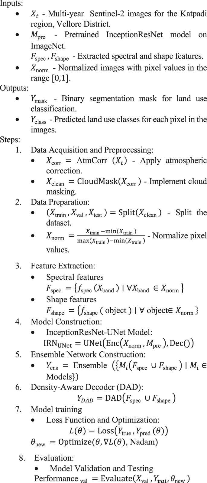
Land use classification using InceptionResNet-UNet and the ensemble network
The multi-year Sentinel-2 images collected from the Katpadi region in the Vellore District are denoted by X-t… These data served as the raw input data for the analysis. The pretrained InceptionResNet model is used as a basic feature extractor; it was first trained on the ImageNet dataset and is denoted by M-pre. The spectral and shape features extracted from the images are denoted by, F-spec and, F-shape.,., respectively, where, F-spec includes spectral characteristics and, F-shape encompasses geometrical and topological features.
The normalized images, with pixel values scaled to the range between 0 and 1, are indicated by X-norm. These normalized images are essential for neural network processing. The outputs of the algorithm include a binary segmentation mask, Y-mask. that indicates land use types at the pixel level and predicted land use classes for each pixel, denoted by Y-class.
After atmospheric corrections are applied to remove distortions, the images are denoted as, X-corr, X-clean. represents the images after cloud masking, which helps avoid misclassification by excluding cloud pixels. The dataset is divided into training, testing, and validation sets, represented by X-train, X-val, X-test, which facilitates different phases of model training, tuning, and evaluation.
The IRUNet architecture is a hybrid model that integrates elements from the UNet and Inception ResNet architectures. It leverages the strength of the InceptionResNetV2 model, a convolutional architecture optimized for image processing tasks, combined with the structural elements of the UNet architecture. The model efficiently processes satellite image processing by extracting and segmenting complex features from images.
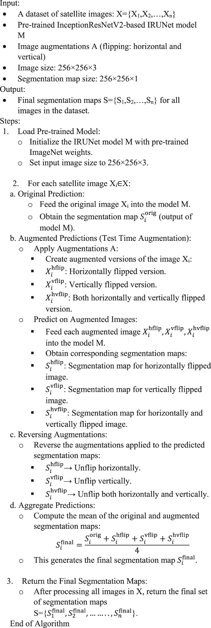
IRUNet with TTA for satellite image segmentation.
InceptionResNet-UNET integration
-
1.
InceptionResNet Model Integration
Let \(X\) represent the input Sentinel-2 images to the network. The InceptionResNet model (Eq. 11), denoted by \({\text{IR}}\left( {X;\theta_{{{\text{IR}}}} } \right)\), processes these images to extract hierarchical features:
$$F_{{{\text{IR}}}} = {\text{IR}}\left( {X;\theta_{{{\text{IR}}}} } \right)$$
(11)
where
-
\(X\) is the input image.
-
\(\theta_{{\text{IR }}}\) represents the parameters of the InceptionResNet model.
-
\(F_{{{\text{IR}}}}\) shows the features extracted by the InceptionResNet model, capturing details at various scales through inception modules.
-
-
2.
U-Net Model for Semantic Segmentation
The U-Net model, denoted as \({\text{UN}}\left( {F_{{{\text{IR}}}} ;\theta_{{{\text{UN}}}} } \right)\), uses the features extracted by the InceptionResNet model to perform semantic segmentation:
$$Y_{{{\text{seg}}}} = {\text{UN}}\left( {F_{{{\text{IR}}}} ;\theta_{{{\text{UN}}}} } \right)$$
(12)
where
-
\(F_{{{\text{IR}}}}\) are the features input into U-Net.
-
\(\theta_{{{\text{UN}}}}\) are the parameters of the U-Net model.
-
\(Y_{{\text{seg }}}\) is the output segmentation mask that delineates land use categories.
-
-
3.
Feature localization and skip connections
The precise localization of features enabled by the skip connections in U-Net can be mathematically represented by linking the feature maps from each encoding layer directly to the corresponding decoding layer. If \(E_{i} \left( {F_{{{\text{IR}}}} } \right)\) and \(D_{i} \left( {Y_{{\text{intermediate }}} } \right)\) represent the \(i^{{\text{th }}}\) encoding and decoding layers, the skip connections are:
$$Y_{{{\text{intermediate }},i}} = D_{i} \left( {Y_{{{\text{intermediate }},i – 1}} \oplus E_{i} \left( {F_{{{\text{IR}}}} } \right)} \right)$$
(13)
where
-
\(\oplus\) denotes the feature map concatenation between the encoder and the decoder.
-
\(Y_{{{\text{intermediate }},i}}\) is the feature map at the \(i^{{\text{th }}}\) level of the decoder.
-
-
4.
Final output layer
The final output layer in U-Net (Eq. 14) uses a convolution to map the decoded features to the segmentation classes:
$$Y_{{\text{final }}} = {\text{Conv}}\left( {Y_{{\text{intermediate,last }}} ;\theta_{{\text{final }}} } \right)$$
(14)
where
-
\(Y_{{\text{final }}}\) is the final binary segmentation mask output.
-
\(\theta_{{\text{final }}}\) are the parameters of the final convolution layer used to generate the segmentation mask.
-
To improve convergence and handle sparse gradients, the Nadam optimizer uses Nesterov momentum and modifies the learning rate according to gradient moments. The detailed hyperparameters are presented in Table 2.
Training and hyperparameters
Loss Function: Dice Loss + Categorical Cross Entropy.
Optimizer: Adam (initial learning rate 1e-4).
Batch Size: 16 Epochs: 150.
Framework: TensorFlow/Keras backend.
Loss function and optimization binary cross-entropy loss:
$$L_{{{\text{BCE}}}} = – \frac{1}{N}\mathop \sum \limits_{{i = 1}}^{N} \left[ {y_{i} \log \left( {p_{i} } \right) + \left( {1 – y_{i} } \right)\log \left( {1 – p_{i} } \right)} \right]$$
(15)
where y is the sample count, t is the true label, and p is the expected probability for the ith sample.
Dice loss
$$L_{{{\text{Dice}}}} = 1 – \frac{{2\mathop \sum \nolimits_{{i = 1}}^{N} y_{i} p_{i} + \epsilon }}{{\mathop \sum \nolimits_{{i = 1}}^{N} y_{i} + \mathop \sum \nolimits_{{i = 1}}^{N} p_{i} + \epsilon }}$$
(16)
Nadam optimizer
$$\theta _{{t + 1}} = \theta _{t} – \eta \frac{{\mathop m\limits^{\prime} _{t} }}{{\sqrt {\mathop v\limits^{\prime} _{t} } + \epsilon }}$$
(17)
where the model parameters are denoted by θ − t, the learning rate is denoted by η, the biased-corrected first and second moment estimates are denoted by m.-t., and ϵ is a tiny constant that prevents division by zero.
Fusion and training
-
1.
Feature extraction
-
\(F_{{\text{IR }}}\) Features are extracted by the InceptionResNet model, which is known for its deep and complex feature extraction capabilities due to its inception modules.
-
\(F_{{{\text{UN}}}}\) Here, features refer to the segmentation outputs from the U-Net model; these features are particularly effective for spatial tasks such as segmentation because U-Net’s architecture features skip connections that help preserve spatial hierarchies in images.
-
-
2.
Feature fusion
-
\(F_{{\text{combined }}}\) The combination of features extracted by InceptionResNet \(\left( {F_{{{\text{IR}}}} } \right)\) (Eq. 18) and the segmentation outputs from U-Net (\(F_{{{\text{UN}}}}\)). This stage is critical since it makes use of InceptionResNet’s thorough feature extraction and U-Net’s exact segmentation capabilities. :
$$F_{{\text{combined }}} = {\text{Fusion}}\left( {F_{{{\text{IR}}}} ,F_{{{\text{UN}}}} } \right)$$
(18)
-
The fusion process aims to integrate diverse and complementary data representations, enhancing the model’s ability to distinguish between different land use types more accurately.
-
Training the network
-
3.
Utilization of combined features for training
-
Training function: Utilizes the combined features, \(F_{{\text{combined }}}\) to train the model (Eq. 19). This function incorporates the selected loss function \(L_{{\text{loss, }}}\), which can be either binary cross entropy (BCE) or Dice loss, based on the data’s properties and the requirements for segmentation:
$$Y_{{\text{predicted }}} = {\text{ Train }}\left( {F_{{\text{combined }}} ,\theta ,L_{{\text{loss }}} } \right)$$
(19)
-
Parameter optimization The Nadam optimizer, an addition to stochastic gradient descent that incorporates Nesterov momentum and sets an adjustable learning rate, is used to optimize the model’s parameters. Highly task-specific, throughout an entire epoch, both the nonconvex and loss function landscape can be quite bumpy at times.
-
The power of the network was augmented by integrating InceptionResNet-UNet architecture into an ensemble network; this way the maximal potential from the strengths of each network has been realized for land use classification.
Technique for test-time augmentation (TTA)
Satellite image processing uses Test Time Augmentation (TTA) to increase the accuracy and reliability of model predictions. At test time, TTA first generates many augmentations of the input images (like flipping or rotating). We then feed these augmented images into the model, averaging predictions from all predicted classes of the original image to arrive at final predictions. This reduces the potential for overfitting, leads to improved generalization of the model, and consequently more reliable results.
TTA is also beneficial for satellite image segmentation with IRUNet, because it can help recognize the complex characteristics in the images, like landform, vegetation, or urban features. Flipping is the most effective TTA method according to experimental results.
Test Time Augmentation (TTA), applied through techniques such as flipping and rotating the images, enhances the robustness of model predictions by reducing overfitting and improving generalization. In satellite image segmentation, where patterns can vary due to lighting, seasonal changes, or geographical features, TTA ensures consistent performance across varying inputs. Experimental results indicated that horizontal and vertical flipping were particularly effective, as demonstrated in Fig. 3, helping the model identify patterns in rotated or mirrored versions of satellite images.

Sample original masked and augmented images. Data Source : NRSC Bhuvan portal—https://bhuvan.nrsc.gov.in Google Earth—https://earth.google.com/web.
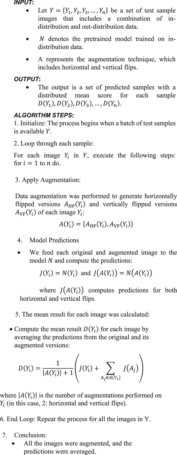
A proposed computational test time augmentation approach is applied to a set of test sample images, denoted as Y = {Y1, Y2, Y3, …, Yn}.
We incorporated test time augmentation (TTA) approaches into the model to improve segmentation performance, which uses model weights to generate numerous predictions from test set images. Figure 3 illustrates the processing pipeline for the original images, horizontal flips, and vertical flips. We enhanced the segmentation result by averaging these projections. We quantitatively evaluated the following performance metrics: precision, recall, Dice similarity coefficient (DSC), area under the precision-recall curve, intersection over union (IoU), and ROC-AUC. We also conducted qualitative assessments to evaluate the visual accuracy of the segmentation results. The models that were considered for training were UNet, ResUNet, Attention-UNet, and the suggested IRU-Net. The following are the key distinctions between these models:
UNet: UNet is characterized by its symmetric encoder-decoder architecture with skip connections that facilitate the flow of context and spatial information.
$${\text{Encoder}}:\;E\left( X \right) = {\text{ReLU}}\left( {MP\left( {CL\left( X \right)} \right)} \right)$$
(20)
$${\text{Decoder}}:\;D\left( Y \right) = {\text{TCL}}\left( {S\left( Y \right)} \right)$$
(21)
Skip Connections: These layers directly concatenate feature maps from encoder layers to corresponding decoder layers, \(S\left({E}_{i}(X)\right)={E}_{i}(X)\) where \(i\) denotes the layer index.
Attention-UNet
By adding an attention mechanism to the skip connections, Attention-UNet expands on UNet by selectively emphasizing key aspects and suppressing less significant information:
$${\text{Attention}}\;{\text{Gate}}:A\left( X \right) = \sigma \left( {{\text{CL}}\left( X \right) \cdot W_{a} } \right)$$
(22)
where σ is the sigmoid function that acts as a gating mechanism and W–a is the weight matrix for the attention layer.
Modified skip connection: The skip connection outputs are modulated by the attention mechanism:
$$S\left( {E_{i} \left( X \right)} \right) = A\left( {E_{i} \left( X \right)} \right) \cdot E_{i} \left( X \right)$$
(23)
ResUNet ResUNet incorporates residual learning into the basic UNet structure, aiming to facilitate training of deeper networks by enhancing gradient flow:
Residual block
$$R\left( X \right) = X + {\text{CL}}({\text{ReLU}}\left( {{\text{CL}}\left( X \right)} \right)$$
(24)
where the letters CL stand for convolutional layers and X represents the input of the residual block.
Integration in the encoder: In each encoder stage, residual blocks are applied, allowing the network to learn identity mappings supplemented with complex features.
IRU-Net To develop IRU-Net, we exploit the properties of both Inception and ResNet for multilevel feature extraction and complex convolutional stacking to capture finer details throughout layers.
Inception-ResNet block
$$E_{{{\text{IR}}}} \left( X \right) = \sum _{k} {\text{CL}}_{k} \left( X \right)$$
(25)
where \(k\) denotes different kernel sizes within the inception module and \({\text{CL}}_{k}\) represents convolutional operations with kernel size \(k\).
UNet integration The encoder of IRU-Net consists of Inception-ResNet blocks, while traditional UNet decoders with skip connections are residual through stages by linking encoded features between the encoder and the decoder. The residual connections used in the InceptionResNetV2 blocks not only help mitigate vanishing gradients but also improve the network’s ability to optimize deep layers. This architecture was chosen due to its success in providing stable training for deep models, especially when dealing with high-resolution satellite imagery that requires multiple levels of abstraction. The UNet preserves high spatial resolution in the segmentation task through progressive upsampling and skip connections while obtaining practical deep feature extraction from its effective encoder. This architecture design enables it to have a better capacity of segmenting fine structures in satellite images like in the urban boundaries or vegetated patterns.