Identifying significant features in adversarial attack detection framework using federated learning empowered medical IoT network security

This study presents a novel AADF-FLEIoTM model. The main intention of the AADF-FLEIoTM model is to improve adversarial attack detection using FL and an advanced hybrid model. To perform that, the AADF-FLEIoTM technique contains data normalization, MPA-based feature selection, attack classification using SA-CNN-BiLSTM, and parameter selection. Figure 1 depicts the workflow of the AADF-FLEIoTM technique.

Data normalization: Min-Max

At first, the data normalization stage executed min-max normalization to scale and transform data into a consistent range²⁹. This model is chosen for scaling data as it usually transforms features to a fixed range [0, 1]. This technique ensures that all features contribute equally to the model, preventing features with more extensive numerical ranges from dominating the learning process. It is specifically effectual when the data is bounded, and the model assumes all features should have a similar scale, such as neural networks or algorithms sensitive to distance metrics. Compared to other methods, namely Z-score normalization, Min-Max is simpler and more intuitive, particularly when the minimum and maximum values of the data are known and consistent. However, it can be sensitive to outliers, a trade-off related to methods less affected by extreme values.

Data standardization is essential for making calculations easier, which the data normalization model achieves. Min-Max normalization is applied to perform the data normalization and is specified as follows:

$$\:S{t}_{B}=\frac{B-{B}_{l}}{{B}_{h}-{B}_{l}}$$

(1)

The data applied to the process is exposed as $\:B$, and the normalized data is presented as $\:S{t}_{B}$. The lowest value is shown as $\:{B}_{l}$, and the highest as $\:{B}_{h}$. Formerly, the essential features were selected from the normalized data utilizing the presented optimization model.

Feature selection process: MPA

For the feature selection process, the proposed AADF-FLEIoTM designs an MPA to identify and retain the most relevant features³⁰. This technique is highly efficient for feature selection as it replicates the search for optimal solutions in a complex search space, making it appropriate for identifying the most relevant features in high-dimensional datasets. Compared to other approaches, MPA is robust against local minima, giving fast convergence, and adapts well to non-linear feature relationships. It also needs fewer parameters to be fine-tuned, which simplifies its implementation. The merit of the MPA model is in its balance between exploration and exploitation, enabling it to efficiently search large feature spaces and improve the performance of ML models. Furthermore, the global search capability of the MPA method outperforms conventional greedy-based methods or simple filters, providing improved accuracy and scalability. Figure 2 describes the steps involved in the MPA method.

A marine predator optimization algorithm is presented using the predominant foraging strategies used by marine predators, especially the Brownian and Levy movement patterns, and the optimum rate of encounter tactics examined in predator-prey biological interactions. The MPA is a population-based model, while the primary solutions, related to those in other meta-heuristic methods, are uniformly distributed through the search space:

$$\:{X}_{0}={X}_{\text{m}\text{i}\text{n}}+rand\left({X}_{\text{m}\text{a}\text{x}}-{X}_{\text{m}\text{i}\text{n}}\right)$$

(2)

Whereas $\:{X}_{\text{m}\text{a}\text{x}}$ and $\:{X}_{\text{m}\text{i}\text{n}}$ represent the lower and upper limits of the variables inside the problem area, $\:rand$ indicates a uniformly distributed random variable range between $\:(0$-1). The optimization process of the model is mainly affected by the Prey and Elite matrices:

$$\:Elite\:={\left[\begin{array}{llll}{X}_{1,1}^{I}&\:{X}_{\text{1,2}}^{I}&\:\dots\:&\:{X}_{1,d}^{I}\\\:{X}_{2,1}^{I}&\:{X}_{2,2}^{I}&\:\dots\:&\:{X}_{2,d}^{I}\\\:\vdots&\:\vdots&\:\ddots\:&\:\vdots\\\:{X}_{n,1}^{I}&\:{X}_{{n}_{{\prime\:}}2}^{I}&\:\dots\:&\:{X}_{\text{n},d}^{I}\end{array}\right]}_{n\times\:d}$$

(3)

$$\:Elite\:={\left[\begin{array}{llll}{X}_{1,1}&\:{X}_{\text{1,2}}&\:\dots\:&\:{X}_{1,d}\\\:{X}_{2,1}&\:{X}_{2,2}&\:\dots\:&\:{X}_{2,d}\\\:\vdots&\:\vdots&\:\ddots\:&\:\vdots\\\:{X}_{n,1}&\:{X}_{{n}_{{\prime\:}}2}&\:\dots\:&\:{X}_{\text{n},d}\end{array}\right]}_{n\times\:d}$$

(4)

Whereas $\:X$ signifies the vector of best predators that is simulated $\:n$ times to make the elite matrix, $\:n$ denotes the size of the population, and $\:d$ represents the solution dimension to the problem. The component $\:Xi$, $\:j$ signifies the $\:jth$ size of the $\:ith$ prey. The matrices Prey and Elite share similar measures.

The optimization procedure of the MPA is structured into three stages, defined by changing speed ratios: the exploration stage, the transitional stage among exploitation and exploration, and the exploitation stage. In the first stage, after the iteration count is below one-third of the maximal iterations. After the speed ratio is higher $\:\left(v\ge\:10\right)$, or after the predator’s velocity surpasses that of the prey, this stage is associated with the initial phases of the optimizer iterations. The mathematic expression for this stage is as shown:

Whereas $\:Iter\:<\frac{1}{3}{\text{M}\text{a}\text{x}}_{-}Iter$

$$\:\overrightarrow{stepsize}={\overrightarrow{R}}_{B}\:\cup\:(\overrightarrow{Elite}-{\overrightarrow{R}}_{B}\cup\:\overrightarrow{Prey}),i=\text{1,2},\dots\:\dots\:n$$

$$\:{\overrightarrow{Prey}}_{\text{i}}={\overrightarrow{Prey}}_{\text{i}}+P\bullet\:\overrightarrow{R}\:\cup\:{\overrightarrow{stepsize}}_{i}$$

(5)

On the other hand, $\:{\overrightarrow{R}}_{B}$ means vector made from arbitrary numbers originating from normal distributions, which characterizes Brownian motion. The $\:\cup\:$ symbol means element-by-element multiplication that is applied to mimic the prey movement by multiplying RB with the prey. Moreover, $\:P$ denotes a constant set at 0.5, whereas $\:\overrightarrow{R}$ refers to a vector of uniform randomly generated numbers in the interval. The term $\:Iter$ relates to the present iteration counts, and $\:{\text{M}\text{a}\text{x}}_{-}$iter represents the maximal iteration counts.

In the next stage of the model, either prey or predators move at a similar speed by a unit speed ratio of 1 $\:\left(v\approx\:\:1\right)$.

Whereas \(\:\frac{1}{3}{\text{M}\text{a}\text{x}}_{-}It\text{e}r.

For the initial half of the population:

$$\:{\overrightarrow{stepsize}}_{\text{i}}={\overrightarrow{R}}_{L}\cup\:\left({\overrightarrow{Elite}}_{\text{i}}-{\overrightarrow{R}}_{L}\cup\:{\overrightarrow{Prey}}_{\text{i}}\right),i=\text{1,2},\dots\:\dots\:\frac{n}{2}$$

$$\:{\overrightarrow{Prey}}_{\text{i}}={\overrightarrow{Prey}}_{\text{i}}+P{\bullet\:}{\overrightarrow{R}}_{L}\cup\:{\overrightarrow{stepsize}}_{\text{i}}$$

(6)

The movement is decided by an arbitrary number vector $\:{\overrightarrow{R}}_{L}$ according to the Lévy distribution, demonstrating Lévy motion. For the next half of the population, the mathematic representation is stated as shown:

$$\:{\overrightarrow{stepsize}}_{\text{i}}={\overrightarrow{R}}_{B}\cup\:\left({\overrightarrow{R}}_{B}\cup\:{\overrightarrow{Elite}}_{\text{i}}-\overrightarrow{Pre{y}_{i}}\right),i=\frac{n}{2},\dots\:\dots\:,n$$

$$\:\overrightarrow{Pre{y}_{i}}={\overrightarrow{Elite}}_{\text{i}}+P\cdot\:CF\cup\:{\overrightarrow{stepsize}}_{\text{i}}$$

(7)

Here, $\:CF={\left(1-\frac{Iter}{{\text{M}\text{a}\text{x}}_{-}ITer}\right)}^{\left(2\frac{Iter}{{\text{M}\text{a}\text{x}}_{-}ter}\right)\:}$ is measured as an adaptive parameter, which controls the step length of the predator. The $\:{\overrightarrow{R}}_{B}$ product and the elite mimic the predator’s movement in Brownian motion, whereas the prey upgrades its location according to this movement. In the third stage of the model, considered by a lower speed ratio $\:(v=0.1)$, the predator travels quicker than the prey. The subsequent mathematical pattern characterizes this stage:

However $\:Iter\:>\frac{2}{3}{\text{M}\text{a}\text{x}}_{-}I$ ter

$$\:{\overrightarrow{stepsize}}_{\text{i}}={\overrightarrow{R}}_{L}\cup\:\left({\overrightarrow{R}}_{L}\cup\:{\overrightarrow{Elite}}_{\text{i}}-{\overrightarrow{Prey}}_{\text{i}}\right),i=\text{1,2},\dots\:\dots\:n$$

$$\:{\overrightarrow{Prey}}_{\text{i}}={\overrightarrow{Elite}}_{\text{i}}+P\cdot\:\text{C}\text{F}\cup\:{\overrightarrow{stepsize}}_{\text{i}}$$

(8)

Environmental aspects, like the formation of vortices or the effects of fish aggregating devices (FADs), can considerably change marine predators’ behaviour. Besides the impact of these features, predators might be required to carry out lengthy leaps through various dimensions to find environments with other prey distributions. FADs can signify local bests inside an exploration region, and setting long leaps in the model optimization procedure can prevent getting stuck in these local ideals. In this regard, FADs represent the probability that affects the model optimizer procedure, generally set at 0.2. $\:\overrightarrow{U}$ denotes a binary vector sequence randomly produced as $\:0$ or 1, whereas $\:r$ denotes a randomly generated number amongst ($\:0$,1). Moreover, $\:{r}_{1}$ and $\:{r}_{2}$ are random indices inside the prey matrix. If$\:\:r\le\:FADs$, predators are involved in long leaps through various dimensions for exploring other best solution areas, thus avoiding local bests. On the other hand, if $\:r\ge\:FADs$, predators move arbitrarily inside the present predator area.

$$\:{\overrightarrow{Prey}}_{\text{i}}=\left\{\begin{array}{l}{\overrightarrow{Prey}}_{\text{i}}+CF\left[{\overrightarrow{X}}_{min}+\overrightarrow{R}\cup\:\left({\overrightarrow{X}}_{\text{m}\text{a}\text{x}}\:-{\overrightarrow{X}}_{min}\right)\right]\cup\:\overrightarrow{U},\:if\:r\le\:FADs\\\:{\overrightarrow{Prey}}_{\text{i}}+\:\left[FADs\:\left(1-r\right)+r\right]\left({\overrightarrow{Prey}}_{r1}-{\overrightarrow{Prey}}_{\text{r}2}\right),\:if\:r>FADs\end{array}\:\:\:\:\:\:\:\:\:\:\:\:\right.$$

(9)

The fitness function (FF) applied in the MPA model is tailored to have a balance among the selected feature counts in all solutions (minimal), and the classification precision (maximal) gained by utilizing these chosen features, Eq. (10) characterizes the FF to assess solutions.

$$\:Fitness=\alpha\:{\gamma\:}_{R}\left(D\right)+\beta\:\frac{\left|R\right|}{\left|C\right|}$$

(10)

Whereas $\:{\gamma\:}_{R}\left(D\right)$ signifies the classification error rate of a provided classifier. $\:\left|R\right|\:$means cardinality of the selected subset, and $\:\left|C\right|\:$denotes total feature counts in the dataset; $\:\alpha\:$ and $\:\beta\:$ are dual parameters related to the significance of subset length and classification quality. ∈ [1,0] and $\:\beta\:=1-\alpha\:.$.

Attack classification: SA-CNN-BiLSTM

Besides, the hybrid SA-CNN-BiLSTM technique is employed for detecting and classifying³¹. This integration provides a robust model for detection and classification tasks, particularly in time-series and sequential data. CNN outperforms extracting spatial features from input data, while BiLSTM captures past and future dependencies, improving the model’s understanding of sequential patterns. Adding Self-Attention allows the model to concentrate on crucial parts of the input sequence, enhancing its capability to capture long-range dependencies and relevant data. This hybrid approach outperforms conventional models by utilizing the merits of each component, presenting improved accuracy and efficiency in detecting complex patterns in data. Compared to simpler models, SA-CNN-BiLSTM is more robust, adaptive, and capable of handling diverse, large-scale datasets with improved performance. Figure 3 depicts the infrastructure of the SA-CNN-BiLSTM model.

A CNN is a multi-layer feedforward NN. A standard CNN method contains an activation layer, convolutional layer, input layer, pooling layer, output layer, and fully connected (FC) layer. The pooling and convolutional layers are frequently arranged in an alternating sequence. The key responsibilities of the layers are defined in the succeeding paragraphs.

Convolutional Layer

The convolutional kernel is the basis for the extraction of features. It removes higher-rank features by exploring input data for convolution processes. This layer is considered by weighted sharing and local awareness. Namely, the weighted matrix is distributed to lessen parameters and reduce the intricacy of the model. The convolutional process is presented in the succeeding Eq. (11):

$$\:{y}_{i}^{l}\left(j\right)={w}_{i}^{l-1}*{x}^{l-1}\left(j\right)+{b}_{i}^{l-1}$$

(11)

Whereas $\:{y}_{i}^{l}\left(j\right)$ denotes the convolution outcome of layer $\:l,{w}_{i}^{l-1}$ represents a weighted matrix of layer $\:l-1$ (the weighted matrix of the $\:i\:th$ convolutional kernel of layer $\:l-1$), and $\:{x}^{l-1}\left(j\right)$ signifies the $\:j\:th$ area where the convolutional process is carried out in layer $\:l-1.$ $\:{b}_{i}^{l-1}$ represents the biased term, which means a bias of the $\:i\:th$ convolutional kernel of layer $\:l-1$. $\:*\:$symbolizes the convolutional process.

The convolution layer uses a pre-defined convolution kernel to implement local convolutions on the input characteristics in step $\:s$. Afterwards, traversal feature mappings are made. For example, a $\:4$x$\:4$ plane was calculated by the $\:3\text{x}3$ convolutional kernel to get a $\:2\text{x}2$ feature mapping. The convolutional kernel parameters are multiplied by the consistent parameters and added to get the values in feature mapping.

Activation Layer

During the CNN’s forward propagation, this layer non-linearly converts the convolutional layer output utilizing an activation function. This mapping of lower-dimension, linearly identical characteristics to large sizes improves the characteristics’ linear separability. Therefore, it enhances the non-linearNN’s approximation and feature extraction ability.

Pooling Layer

This layer is tailored to decrease calculation during this CNN by condensing the feature sizes. It establishes the high-order characteristics removed by the convolutional layer, enhances the networking iteration efficacy, and gives the characteristics with translation invariance. The standard pooling models contain max pooling, which captures the maximal value in the perceptive area, and average pooling, which captures an average value. The succeeding equations are applied,

$$\:{y}_{i,j,k}^{l}=\text{m}\text{a}\text{x}\left\{{x}_{i,j,k}^{l},s\right\}$$

(12)

$$\:{y}_{i,j,k}^{l}=\frac{1}{N}\sum\:{x}_{i,j,k}^{l}$$

(13)

Whereas $\:{y}_{i,j,k}^{l}$ denotes $\:k\:th$ feature mapping output in the $\:l\:th$ layer, $\:{x}_{i,j,k}^{l}$ symbolizes $\:(i,j)th$ module in the $\:kth$ feature mapping output from $\:the\:lth$ convolutional layer.

The LSTM method, a recurrent neural network (RNN), is presented to overcome the normal gradient explosion and vanishing problems in RNNs. An LSTM method can learn and preserve temporal and sequential patterns in longer sequences. Compared with conventional RNNs, LSTM models rely on gate mechanisms and present input, output, and forgetting gates derived from an RNN, which controls the flow of information over the gating mechanism. Bi-LSTM expands the conventional LSTM method, which enhances the model performance in processing sequential issues. A Bi-LSTM technique relates an LSTM method in either direction. Over its bi-directional architecture, the network’s output layer can effectively use the state data of the preceding moment to create complete data usage. The Bi-LSTM network’s backward and forward layers handle the sequences individually, and next, the dual outputs pre and post were merged to get the last output outcome. Bi-LSTM is applied utilizing the succeeding equations:

$$\:\overrightarrow{{h}_{t}}=LSTM(\overrightarrow{{h}_{t-1}},{x}_{t})$$

$$\:\overleftarrow{{h}_{t}}=LSTM\left(\overrightarrow{{h}_{t+1}},{x}_{t}\right)$$

(14)

$$\:{h}_{t}=\left[\overrightarrow{{h}_{t}},\overleftarrow{{h}_{t}}\right]$$

Whereas $\:{h}_{t}$ characterizes the $\:output\leftarrow\:$ of the output layer at $\:tth$ time$\:\overrightarrow{{,\:h}_{t}}$ and $\:\overleftarrow{{h}_{t}}$ characterize the output of the forward and reverse layer at $\:tth$ time$\:,$ and $\:{x}_{i}$ characterizes an input$\:.$.

The AM was initially presented using this method. It mimics human vision and splits dissimilar areas with several weights to illustrate the difference. AM has recently been extensively applied in the domain of DL because it can strengthen main information and weaken incorrect data. The computation method for the AM is separated into 3 phases. In the initial phase, the attention score related to all keys is gained by computing the similarities between the key and the query. In this second phase, the attention scores are standardized utilizing the function of Softmax to get the weight coefficients. In the third phase, dissimilar weighting coefficients are summed and weighted to underline the main information and disregard insignificant details. The equations are stated below.

$$\:F\left(Q,{K}_{i}\right)={Q}^{T}\cdot\:K$$

$$\:{a}_{i}=softmax\left(F\left(Q,{K}_{i}\right)\right)=\frac{\text{e}\text{x}\text{p}\left(F\left(Q,{K}_{i}\right)\right)}{{\varSigma\:}_{i=1}^{l}\text{e}\text{x}\text{p}\left(F\left(Q,{K}_{i}\right)\right)}$$

(15)

$$\:A\left(Q,K,\:V\right)={\sum\:}_{i=1}^{l}{a}_{i}\cdot\:{V}_{i}$$

$\:Q$,$\:\:K,$ and $\:V$ denote query, key, and numerical matrix, and $\:{a}_{i}$ represents weighting coefficients. If $\:Q=K=V$, the AM becomes a self-AM.

Hyperparameter tuning: RTH optimizer algorithm

Finally, the RTH optimizer algorithm optimally adjusts the hyperparameter values of the SA-CNN-BiLSTM model, resulting in more excellent classification performance³². This model was chosen due to its nature-inspired exploration-exploitation balance, which makes it highly effective for optimization tasks. The algorithm replicates the predatory behaviour of hawks, allowing it to explore vast search spaces while refining solutions through targeted exploitation. Compared to conventional optimization methods like grid search or gradient-based techniques, RTH can handle complex, non-linear, and multi-modal problems better. Its capability to adapt dynamically to diverse problem landscapes improves its robustness and efficiency in tuning model hyperparameters. Furthermore, RTH is less likely to get trapped in local optima, giving a more global search strategy and yielding better results, particularly in high-dimensional spaces. This flexibility and resilience make RTH a robust choice over other techniques. Figure 4 demonstrates the structure of the RTH approach.

In general, the conventional and mathematical optimizer models frequently fail to acquire the best values of the systems. Besides, metaheuristic optimizations (MHO) play a significant part, which is recognized in modern optimizers due to recent and new methods. Considerably, optimizations are commonly categorized as per their resource of inspiration. The RTH optimizer is a swarm intelligence optimizer tool. It has shown its efficacy in managing non-linear and intricate behaviour issues. It was chosen because of the RTH model’s efficiency and novelty. The complete details of the RTH optimizer are given below:

RTH is a greedy bird that uses hunt and attack tactics to hunt for prey. These strategies begin with the detection procedure and finish with the swooping procedure. Furthermore, hunting includes three phases: high-soaring, low‐soaring, and swooping. The initialization procedure is considered the initial step for every SI optimizer, which is answerable for making the initial future solution at random. The initial solutions are produced utilizing the below-mentioned formulation:

$$\:{\chi\:}_{i}^{d}={L}_{i}^{d}+\left({U}_{i}^{d}-{L}_{i}^{d}\right)*{r}_{i}^{d}$$

(16)

Here, $\:x$ denotes the produced initial value for $\:ith$ solution in dimension $\:d$; the lower limit is denoted as $\:L$, and the upper limit is represented as $\:U$ utilizing a randomly produced generator, $\:r.$

After the solutions are set, they serve an objective function for assessing the position of global best, $\:{x}_{G}$, and for computing an average value, $\:{x}_{av}$. Next, they are upgraded over the three above-mentioned tactics.

High soaring

At this phase, the RTH flies far away from its prey to discover the finest position. This phase is mathematically formulated below:

$$\:x\left(k\right)={\chi\:}_{G}+\left({x}_{av}-x\left(k-1\right)\right).\:Levy\left(Dim\right)\cdot\:TF\left(k\right)$$

(17)

Here, $\:x\left(k\right)$ denotes the position of RTH; $\:{x}_{G}$ represents the global best location; $\:{x}_{av}$ indicates an average of every area at $\:the\:kth$ iteration. $\:Levy$ represents the function of levy flight distribution; $\:TF\left(k\right)$ represents the function of the transition factor.

$$\:Levy\left(Dim\right)={C}_{1}\frac{{r}_{1}\cdot\:\sigma\:}{|{r}_{2}{|}^{{C}_{2}^{-1}}}$$

$$\:\sigma\:=\left(\frac{\varGamma\:\left(1+{C}_{2}\right).\cdot\:\text{sin}\left(\frac{\pi\:{C}_{2}}{2}\right)}{\varGamma\:\left(\frac{1+{C}_{2}}{2}\right){C}_{2}2\left(\frac{1-{C}_{2}}{2}\right)}\right)$$

(18)

While $\:{C}_{1}$ and $\:{C}_{2}$ refer to a constant of 0.01 and 1.5, respectively, $\:Dim$ means an unknown variable (dimension); $\:{r}_{1}$ and $\:{r}_{2}$ are dual variables, generating values randomly from $\:0$ to 1.

$$\:TF\left(k\right)=1+sin\left(2.5+\left(\frac{k}{{T}_{m}}\right)\right)$$

(19)

Here, $\:{T}_{m}$ signifies the maximum iteration count.

Low soaring

The hawk soars far nearer to its pointed prey in a curved drive to encircle it. This method is formulated below:

$$\:x(k+1)={x}_{G}+\left(x\right(k)+y(k\left)\right)\cdot\:{T}_{s}\left(k\right)$$

$$\:{T}_{s}\left(k\right)=x\left(k\right)-{x}_{av}$$

(20)

Meanwhile, $\:x$ and $\:y$ signify the direction coordinates. The formulation to compute them is exposed below:

$$\:\left\{\begin{array}{l}x\left(k\right)=A\left(k\right)\cdot\:sin\left(\theta\:\right(k\left)\right)\\\:\left(17\right)\\\:y\left(k\right)=A\left(k\right)\cdot\:cos\left(\theta\:\right(k\left)\right)\end{array}\right.\left\{\begin{array}{c}A\left(k\right)={A}_{0}.\left(g-\frac{k}{km{T}_{m}}\right).{r}_{3}\\\:\theta\:\left(k\right)=\varnothing\:\left(1-\frac{k}{T}\right).{r}_{3}\end{array}\right.\left\{\begin{array}{l}x\left(k\right)=\frac{x\left(k\right)}{\text{m}\text{a}\text{x}\left|x\right(k\left)\right|}\\\:y\left(k\right)=\frac{y\left(k\right)}{\text{m}\text{a}\text{x}\left|y\right(k\left)\right|}\end{array}\right.$$

Here, $\:{A}_{0}$ indicates an initial value within the range from 0.5 to 3, $\:\varnothing\:$ represents the angel gain within the range from 5 to 15, $\:{r}_{3}$ denotes a produced variable randomly within an interval from [ $\:0$ to 1], $\:g$ denotes a controlling parameter from the range [1 to 2].

Stooping and Swooping

In this stage, the hawk shortly bends and subsequently attacks its prey. It is recognized for attaining the finest location over the low-soaring stage. Precisely, this tactic is formulated below:

$$\:x\left(k\right)=\alpha\:\left(T\right)\cdot\:{x}_{G}+x\left(k\right)\cdot\:{T}_{\$1}\left(k\right)+y\left(T\right)\cdot\:{T}_{s2}\left(k\right)$$

(21)

The steps’ dimensions are attained as per the:

$$\:{T}_{s1}\left(k\right)=x\left(k\right)-rF\left(k\right)\cdot\:{x}_{av}$$

$$\:{T}_{s2}\left(k\right)=G\left(k\right)\cdot\:x\left(k\right)-TF\left(k\right)\cdot\:{x}_{G}$$

(22)

where $\:G$ and $\:\alpha\:$ denote the gravitational and accelerating parameters correspondingly. The mathematical formulations are given below:

$$\:\alpha\:\left(k\right)=si{n}^{2}\left(2.5-\frac{k}{{T}_{m}}\right)$$

$$\:G\left(k\right)=2\cdot\:\left(1-\frac{k}{{T}_{m}}\right)$$

(23)

Algorithm 1 illustrates the RTH model.

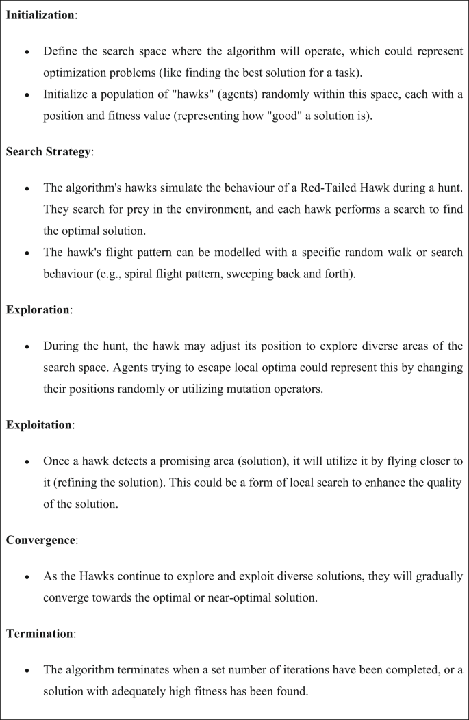
In the above equation, $\:\alpha\:$ represents the accelerator factor for speeding up the convergence procedure. Moreover, $\:G$ represents the gravitational effect, which is reduced slowly when the hawk is far nearer to the prey for pretending the exploitation stage. The RTH model originates an FF to achieve a boosted classification performance. It establishes an optimistic number to symbolize the better outcome of the candidate’s solutions. In this paper, the reduction of the classification error rate was reflected as the FF, as provided in Eq. (24).

$$\:fitness\left({x}_{i}\right)=ClassifierErrorRate\left({x}_{i}\right)\:=\frac{no.\:of\:misclassified\:samples}{Total\:no.\:of\:samples}\times\:100$$

(24)

Source link