Global emission factor dataset for Scope 3 machine learning applications

In this section, we first introduce the core concepts of Environmentally Extended Multiregional Input-Output (EE-MRIO) analysis and explain why it underpins most emission-factor datasets in ecological economics research. We then compare five major EE-MRIO datasets—WIOD, GTAP, Eora, USEEIO, and Exiobase—highlighting their accessibility, coverage, time horizon, sector detail, and types of emission factors. Next, we demonstrate how ExioML was constructed as an open-source emission-factor dataset (EFDB) derived from ExioBase 3.8.2. We describe the construction workflow, the factor tables, the footprint networks, and the GPU-accelerated toolkit used to generate the released files.

EE-MRIO as a Foundation for Emission-Factor Datasets. Environmentally Extended Multiregional Input-Output (EE-MRIO) analysis frames the global economy as a network of interlinked sectors spanning multiple regions^{16,17,18,19,20}. It builds on classical work in interregional and international input-output modelling, which first formalised the idea of a space-economy in which regions are connected through trade and production linkages^21,22. Traditional input-output models focus on monetary flows among sectors, while their environmentally extended variants incorporate resource use and pollutant emissions^{18,23,24,25,26}. As Fig. 1 shows, an EE-MRIO dataset typically includes:

• A transaction matrix (Z) that records monetary flows between sectors and captures how industries purchase inputs from one another.

• A final demand matrix (Y) capturing non-intermediate consumption by households, government, and international markets (including exports).

• One or more factor accounts (F) specifying emissions and resource use by sector, containing environmental extensions such as GHG emissions, resource extraction, and pollutant releases.

By combining Z, Y, and F, researchers can trace embodied emissions through complex supply chains, thereby calculating the total (direct + indirect) impact of any given sector. This approach underpins many studies of consumption-based accounting and trade-linked pollution, where emissions are allocated to the final consumers who drive production^27,28. It also informs structure-decomposition analysis²³ and sustainability evaluations in global trade^29,30. Methodological introductions such as Kitzes provide accessible overviews of how environmentally extended input-output analysis connects economic accounts with environmental extensions and footprint indicators²⁶.

Machine learning (ML) has recently entered the EE-MRIO arena for tasks such as automatically identifying high-emission hotspots and optimizing logistics³¹. Recent surveys show that machine learning can be a powerful tool for reducing greenhouse gas emissions and aiding society’s adaptation to climate change³². These works highlight how ML can complement EE-MRIO frameworks by automating hotspot detection, scenario forecasting, and anomaly identification. Embedding high-dimensional input-output data to discover latent patterns in supply chains^33,34, forecasting future emissions based on economic or technology scenarios^12,13, and clustering industrial sectors by environmental similarity for policy design^35,36 are all active research directions. Each of these tasks requires robust, well-documented EE-MRIO data.

However, these ML applications critically depend on open, granular, and up-to-date emission factors that map sector-level outputs to GHG intensities. In practice, many existing EE-MRIO datasets have restrictions or incomplete coverage, limiting reproducibility and cross-study benchmarking. Earlier work on building multi-year MRIO systems—for example the embedded carbon emissions indicator for the UK, constructed via an MRIO data optimisation system³⁷—demonstrates both the analytical value and the practical complexity of assembling time series of harmonised input-output tables. ExioML builds on these methodological strengths and formats the resulting emission factors for ML pipelines.

Comparison of Major EE-MRIO Datasets.Table 2 summarizes five commonly used EE-MRIO datasets and contrasts them with our proposed ExioML. Each dataset has distinctive strengths, yet also presents certain limitations when viewed from an ML perspective.

Accessibility and Licensing. While WIOD and Exiobase are nominally free, GTAP requires paid licenses, and Eora’s highest-resolution tables can also be costly to acquire. In contrast, ExioML retains Exiobase’s open-access basis and distributes ready-to-use factor tables in user-friendly formats.

Coverage & Updates. Eora is highly granular and frequently updated, but not fully open. GTAP covers a large set of regions but only releases discrete “snapshot” versions every few years, limiting time-series forecasting. WIOD’s coverage ends around 2016. ExioML extends Exiobase’s coverage to 2022, enabling more recent analyses of trends.

Sector Detail & Emissions Scope. Some datasets track only energy-related CO₂, whereas ExioML inherits thousands of environmental categories from Exiobase (417 emission types, 662 resource types). This breadth is vital for advanced ML tasks that go beyond carbon, e.g., analyzing air pollutants, water use, or material footprints.

Implications for ML. The standardized formats and coverage enable reuse in benchmarking and downstream analyses, subject to the constraints noted in the dataset description.

Machine-learning formulation. ExioML is organized to support machine-learning workflows in which sector attributes and network-derived features are used to estimate emission factors. The motivation for ML is practical: full EE-MRIO tables are high-dimensional and costly to recompute, while many applications require rapid estimation, imputation, or cross-year prediction on standardized features. The tabular and edge-list releases allow studies to operate without reconstructing full MRIO matrices.

Regression setting. We frame the primary tasks as supervised regression, with inputs drawn from the Factor Accounting tables (e.g., value added, employment, energy totals) and optional features derived from the Footprint Networks. The targets are continuous emissions or intensities (e.g., kg CO₂-eq), making regression a natural formulation; classification uses, when needed, thresholds or bins applied to these continuous targets. Region, sector, and year provide categorical or ordinal covariates alongside numeric attributes.

Input representation. The Factor Accounting tables provide numeric attributes and categorical identifiers that are directly usable in tabular pipelines. The Footprint Network edge lists can be consumed as graph inputs or aggregated into node-level summaries (e.g., inflow and outflow totals) before modeling. This separation supports both tabular and graph-based learning under a consistent schema.

Model families. We distinguish statistical machine-learning models, which rely on explicit features and comparatively shallow function classes (e.g., linear models, nearest neighbors, or tree ensembles), from deep learning models that learn hierarchical representations through multi-layer neural networks or attention mechanisms. This distinction captures differences in representation learning and capacity rather than data provenance. The Technical Validation section evaluates representative models from both families using the released ExioML tables.

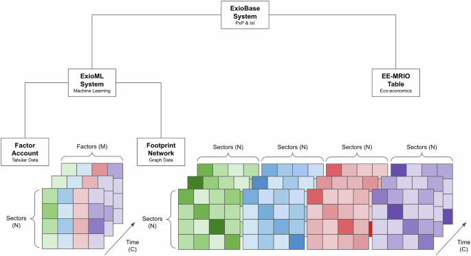
Building ExioML as an Open Emission-Factor Dataset. The proposed ExioML dataset is an emission-factor dataset built by carefully restructuring the raw Exiobase 3.8.2 files. Figure 2 outlines the system architecture. We preserve the comprehensive environmental accounting of Exiobase but reformat it into two user-facing components:

• Factor Accounting (Tabular Data): Provides sector-level measures such as value added, employment, energy consumption, and total GHG emissions. These can be viewed as emission factors under different normalizations, e.g. per monetary unit or per unit of output.

• Footprint Networks (Graph Data): Graph-based representations of inter-sector trade flows annotated with embodied emissions capture the full trading network across 49 regions. Each edge denotes inter-sector flows and can store derived footprints of various pollutants.

ExioBase 3.8.2 itself comprises over 40 GB of supply-use tables, satellite accounts, and emission categories^15,38. Users lacking deep input-output expertise often find it difficult to extract the relevant portion for machine learning tasks. To mitigate this challenge, we developed a GPU-accelerated toolkit that loads Exiobase, performs the required matrix operations, and outputs a compressed edge table or factor table for each year from 1995 to 2022. Data extraction and MRIO operations build on the open-source pymrio toolbox³⁸. It provides automated download and parsing routines for EXIOBASE and related EE-MRIO datasets. In constructing ExioML from over 40 GB of raw EE-MRIO files, we identify three main challenges that must be overcome to enable scalable machine-learning-ready emission-factor extraction:

1. 1.

   Large-scale matrix computation: We implement the Leontief-based footprint calculation with CUDA or equivalent GPU libraries, accelerating (I−A)⁻¹y multiplications that would otherwise be prohibitively slow on standard CPUs.

2. 2.

   Sparse representation of trade networks: Instead of storing a 200 × 200 adjacency for every region pair, we keep only the top million edges per year that exceed a threshold flow, reducing file size.

3. 3.

   Standardized units and naming conventions: We unify currency units, sector codes, and emission categories to ensure direct comparability across all 49 regions and 28 time steps.

Openness and license compliance. ExioML is built solely from the openly available EXIOBASE 3.8.2 dataset, which is distributed under the Creative Commons Attribution–ShareAlike 4.0 International (CC BY-SA 4.0) license. This license permits reuse and redistribution with attribution and a share-alike obligation; ExioML follows these terms by releasing derived factor and footprint tables under a compatible open licence. No proprietary MRIO inputs (e.g., GTAP or full-resolution Eora tables) are incorporated; they are cited only for contextual comparison. EXIOBASE can be accessed via Zenodo and European Environment Agency portals, and we follow the data providers’ recommended citations^15,38.

The overall workflow is consistent with established practice in constructing multi-regional input-output systems and associated footprint indicators, such as the time-series MRIO for embedded carbon emissions developed for the UK³⁷ and subsequent global carbon-footprint studies based on trade-linked MRIO models²⁸.

Emission Factors in ExioML. The details of ExioML are summarised in Table 3. Four essential factors included in ExioML are identified by the EE research community: GHG emissions, population, gross domestic product (GDP), and total primary energy supply (TPES), the total energy available for use in an economy from all primary sources. The decomposition uses the Kaya Identity²⁴. This identity expresses emissions as the product of population, affluence, energy intensity, and carbon intensity, and was designed specifically for climate-change analysis. This method breaks down carbon emissions into four indicators, which are population (P), GDP per capita (G/P), energy intensity (E/G) and carbon intensity (F/E):

Beyond the Kaya identity, structural decomposition analysis (SDA) offers a general framework for attributing changes in environmental indicators to driving forces such as technology, demand, and structural effects. Prior work provides comprehensive discussions of alternative decomposition techniques for policymaking in energy and environmental applications³⁹ and highlights the trade-offs between different SDA formulations. A comparative review of SDA and index decomposition analysis outlines their respective strengths in input-output studies²³.

Technical Details of EE-MRIO Computations. Following standard EE-MRIO notation, let Z be the global transaction matrix (block-partitioned by region) and Y the final-demand matrix. Let x be the global output vector, such that

We compute the direct-requirement matrix \(A=Z{\widehat{x}}^{-1}\), which shows how much input each sector requires from others per unit of output. From this, the Leontief inverse L = (I−A)⁻¹ is obtained, capturing the total direct and indirect production requirements across the entire supply chain. For a factor F (e.g., sector-level GHG emissions), we define the intensity vector \(S=F{\widehat{x}}^{-1}\) to represent emissions or resource use per unit of economic output. The final footprint D, the total embodied emissions driven by final demand across all regions and sectors, is computed as

where y collects final demand by region. This standard formulation underlies many MRIO-based footprint and consumption-based accounting studies, including national and global carbon-footprint analyses that link territorial emissions, trade, and final consumption^28,37.

PxP and IxI Variants. Exiobase 3.8.2 is distributed in two classifications. The product-by-product (PxP) version organises flows by 200 product categories, whereas the industry-by-industry (IxI) version describes flows between 163 industrial sectors. For maximum flexibility, ExioML retains both versions:

• PxP: Suitable for analyzing product-level footprints (e.g., food, textiles, chemicals) in more detail.

• IxI: Appropriate for policy or managerial studies focusing on industries (e.g., agriculture, manufacturing, retail).

Both follow the same data-structure pattern so that ML researchers can train on PxP and validate on IxI to test model generalization. Table 3 summarizes key details of the ExioML dataset. Toolkit Implementation and Availability. Our open-source ExioML development toolkit lowers technical barriers by:

• Performing heavy data preprocessing: discarding unnecessary satellite accounts, ensuring consistent units, labeling sector codes.

• Storing multi-dimensional networks in a single edge table with memory-efficient compression.

• Exposing a simple Python package to query any combination of the 417 emission categories and 662 resources available in Exiobase.

• Providing optional GPU-accelerated modules for matrix inversion and footprint calculations.

The data are available on Zenodo along with documentation and scripts to recreate the factor tables⁴⁰. This standardization supports reproducibility and provides a basis for future updates to ExioML.