Exploring unsupervised learning metrics – KDnuggets

Image by rawpixel from Freepik

Unsupervised learning is a branch of machine learning in which the model learns patterns from available data rather than being provided with actual labels. Let the algorithm come up with the answer.

There are two main techniques for unsupervised learning. Clustering and dimensionality reduction. Clustering techniques use algorithms to learn patterns and segment data. In contrast, dimensionality reduction techniques try to reduce the number of features by keeping the real information as intact as possible.

An example algorithm for clustering is K-Means and an algorithm for dimensionality reduction is PCA. These were the most commonly used algorithms in unsupervised learning. However, we rarely talk about metrics for evaluating unsupervised learning. This is useful, but we need to evaluate the results to know if the output is accurate.

This article describes metrics used to evaluate unsupervised machine learning algorithms and divides them into two sections. Clustering algorithm metrics and dimensionality reduction metrics. Let’s get into it.

I won’t go into detail on the clustering algorithm as it’s not the main point of this article. Instead, we will focus on examples of metrics used for evaluation and how the results are evaluated.

This article uses Kaggle’s Wine dataset as an example dataset. Let’s first read the data and use the K-Means algorithm to segment the data.

import pandas as pd
from sklearn.cluster import KMeans
df = pd.read_csv('wine-clustering.csv')

kmeans = KMeans(n_clusters=4, random_state=0)
kmeans.fit(df)

Start cluster as 4. That is, split the data into four clusters. Is there a good number of clusters? Or is there a better cluster number? In general, you can use a technique called Elbow method Find a suitable cluster. Below is the code.

wcss = []
for k in range(1, 11):
    kmeans = KMeans(n_clusters=k, random_state=0)
    kmeans.fit(df)
    wcss.append(kmeans.inertia_)

# Plot the elbow method
plt.plot(range(1, 11), wcss, marker="o")
plt.xlabel('Number of Clusters (k)')
plt.ylabel('WCSS')
plt.title('Elbow Method')
plt.show()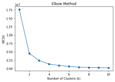

The elbow method uses WCSS or Within-Cluster Sum of Squares to compute the sum of squared distances between various k (cluster) data points and their respective cluster centroids. The best k value is expected to be the one with the greatest decrease in WCSS, or the elbow (2) in the figure above.

However, we can extend the elbow method to find the optimal k using other metrics. What about an algorithm that automatically finds the cluster number without depending on centroids? Yes, it can also be evaluated using a similar metric.

As a note, even without using the K-Means algorithm, you can assume the centroid as the data mean for each cluster. Therefore, algorithms that did not rely on centroids during data segmentation can still use centroid-dependent metric evaluations.

silhouette coefficient

Silhouette is a clustering technique that measures the similarity of data within a cluster relative to other clusters. The Silhouette Coefficient is a numeric representation that ranges from -1 to 1. A value of 1 means that each cluster is completely different from the other clusters, and a value of -1 means that all data was assigned to the wrong cluster. 0 means there are no meaningful clusters from the data.

You can use the following code to calculate the silhouette factor.

# Calculate Silhouette Coefficient
from sklearn.metrics import silhouette_score

sil_coeff = silhouette_score(df.drop("labels", axis=1), df["labels"])
print("Silhouette Coefficient:", round(sil_coeff, 3))

Silhouette coefficient: 0.562

We can see that the above segmentation has a positive silhouette coefficient. This means that there is some isolation between clusters, but some overlap still occurs.

Kalinsky-Halabas Index

The Calinski-Harabasz Index, or Variance Ratio Criterion, is an index used to assess cluster quality by measuring the ratio of between-cluster variance to within-cluster variance. Basically, we measured the difference in the sum of the squared distances of the data between the data in the cluster and the inner cluster.

Higher Calinski-Harabasz Index scores mean better separation of clusters. However, the open-ended score means that the metric is better suited for evaluating different k numbers rather than just interpreting the results.

Let’s calculate the Calinski-Harabasz Index score using Python code.

# Calculate Calinski-Harabasz Index
from sklearn.metrics import calinski_harabasz_score

ch_index = calinski_harabasz_score(df.drop('labels', axis=1), df['labels'])
print("Calinski-Harabasz Index:", round(ch_index, 3))

Kalinsky-Halabas Index: 708.087

Another consideration for the Calinski-Harabasz Index score is that the score is affected by the number of clusters. A higher number of clusters can result in a higher score. Therefore, we recommend using other indicators alongside the Calinski-Harabasz Index to validate your results.

Davis Boldin Index

The Davies-Bouldin Index is a cluster evaluation metric measured by calculating the average similarity between each cluster and its most similar clusters. Similarity is calculated by the ratio of intra-cluster distance to inter-cluster distance. This means that the farther apart the clusters are, the lower the variance, the higher the score.

In contrast to previous indexes, the Davies-Bouldin Index aims for the lowest possible score. The lower the score, the more separated each cluster. Let’s calculate the score using a Python example.

# Calculate Davies-Bouldin Index
from sklearn.metrics import davies_bouldin_score

dbi = davies_bouldin_score(df.drop('labels', axis=1), df['labels'])
print("Davies-Bouldin Index:", round(dbi, 3))

Davis-Boldin Index: 0.544

Similar to the above metric, we cannot say that the above score is good or bad, because we need to use various metrics as support to evaluate the results.

Unlike clustering, dimensionality reduction aims to reduce the number of features while preserving the original information as much as possible. As such, many of the metrics for dimensionality reduction have been about information preservation. Let’s reduce the dimensionality using PCA and see how the metric works.

from sklearn.decomposition import PCA
from sklearn.preprocessing import StandardScaler

#Scaled the data
scaler = StandardScaler()
df_scaled = scaler.fit_transform(df)

pca = PCA()
pca.fit(df_scaled)

In the example above, we have fitted PCA to the data, but have not yet reduced the number of features. Instead, we want to evaluate the trade-off between dimensionality reduction and variance. Cumulative explanatory varianceSeeing how information remains in each feature reduction is a common metric for dimensionality reduction.

#Calculate Cumulative Explained Variance
cev = np.cumsum(pca.explained_variance_ratio_)

plt.plot(range(1, len(cev) + 1), cev, marker="o")
plt.xlabel('Number of PC')
plt.ylabel('CEV')
plt.title('CEV vs. Number of PC')
plt.grid()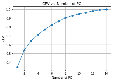

From the chart above, we can see the amount of PCs retained compared to the explained variance. As a rule of thumb, when attempting dimensionality reduction, we often choose to keep around 90-95%, so following the chart above will reduce around 14 features to 8.

Let’s look at other metrics to validate the dimensionality reduction.

reliability

Reliability is a measure of the quality of a dimensionality reduction technique. This metric measured how well the reduced dimensionality retained the nearest neighbors of the original data.

Basically, the metric tries to see how well the dimensionality reduction technique preserves the data in preserving the local structure of the original data.

The reliability metric ranges from 0 to 1, with values ​​closer to 1 meaning that the closest neighbors to the data point in the reduced dimension are also nearly as close in the original dimension.

Let’s calculate the reliability metric using Python code.

from sklearn.manifold import trustworthiness

# Calculate Trustworthiness. Tweak the number of neighbors depends on the dataset size.
tw = trustworthiness(df_scaled, df_pca, n_neighbors=5)
print("Trustworthiness:", round(tw, 3))

Confidence: 0.87

summon mapping

Sammon’s mapping is a nonlinear dimensionality reduction technique for preserving high-dimensional pairwise distances during reduction. The goal is to compute the pairwise distance between the original data and the reduced space using Sammon’s stress function.

A lower Sammon stress function score is better because it indicates better pairwise preservation. Let’s use the Python code example.

First, install additional packages for Sammon’s Mapping.

pip install sammon-mapping

Then use the following code to calculate Sammon’s stress:

# Calculate Sammon's Stress
from sammon import sammon

pca_res, sammon_st = sammon.sammon(np.array(df))

print("Sammon's Stress:", round(sammon_st, 5))

Summon’s Stress: 1e-05

As a result, we found that the Sammon’s score was low and the data was preserved.

Unsupervised learning is a branch of machine learning that attempts to learn patterns from data. Output evaluation is sometimes less discussed compared to supervised learning. In this article, we will try to learn some unsupervised learning metrics such as:

1. Within-Cluster Total Square
2. silhouette coefficient
3. Kalinsky-Halabas Index
4. Davis Boldin Index
5. Cumulative explanatory variance
6. reliability
7. summon mapping

Cornelius Judah Wijaya is a data science assistant manager and data writer. While working full-time at Allianz Indonesia, he loves sharing his Python and data tips through social and writing media.