Trial design
The current research was intended to be a clinical trial. This research was authorized by the Deraya University Ethical Committee (No: 17/2023). According to the Helsinki Declaration’s ethical standards. This study adheres to human research principles. Following a full explanation of the trial, all participants signed a written consent form. From February 2023 until July 30th, 2023, the trial was held at a medical clinic for outpatients.
The sample size
To prevent type II error, a sample size calculation was performed before the study using the G*Power (Wilcoxon–Mann–Whitney test)25. This output displays the results of an a priori power analysis for a linear regression t-test. The purpose is to determine the minimum required sample size needed to achieve a desired statistical power of 0.95 (95%).
Specifically:
-
A one-tailed t-test is specified to detect an alternative slope (H1) of 0.1732051 as greater than the null slope of 0.
-
An alpha error probability of 0.05 is set.
-
The desired power is 0.95, with standard deviations and null/alternative slopes provided.
The analysis calculates a no centrality parameter δ of 3.3665016 based on these inputs.
It then determines the critical t-value of 1.6938887 and degrees of freedom of 32 needed to achieve ≥ 0.95 power. The total required minimum sample size to meet these conditions is calculated as 34 observations. The actual estimated power computed from these parameters is 0.9504455, exceeding the target of 0.95 power. Therefore, this output provides the minimum sample size (N = 34) required to have a 95% chance of correctly detecting a statistically significant slope of 0.1732051 in a one-tailed linear regression t-test at the 5% significance level. This means that the study has enough power to identify a significant difference between the two measures with high confidence. As a result, the study has an acceptable sample size, and the results are reliable and genuine.
Participants
The sixty-three participants in the research study were initially diagnosed with abdominal obesity and recruited from the clinical nutrition department of the General Hospital. Recruitment was based on the following criteria: females and males participated in this trial; their ages varied from 25 to 45 years, their BMI was 25–29.9 kg/m2, and the participants were not treated with lipolytic drug therapy.
Exclusion criteria
Any prior medical history of cardiopulmonary disease, disc prolapse, disease of the liver or kidneys, gastric or gallbladder ulcer, diabetes mellitus, cigarette smoking, cognitive impairments, patients who have peacemaker or any type of metal implant on the treated area, cancer or patients with a history of tumor and any surgery related to the spine, abdomen, or pelvis.
Outcome measures
All of the participants were evaluated before and after two months of intervention, with two sessions each week. Anthropometry is the measurement of one’s weight, height, waist circumference, and calculated BMI.
Waist circumference
Non-elastic, tight, and 150-cm tape is used. The distance was measured midway between the base of the lower rib and the top of the iliac crest. Waist circumference is an indicator of central obesity, which is where adipose tissue is deposited4.
Body mass index
The body mass index (BMI) for all participants was calculated using the following equation using a universal height-weight scale to ascertain the subject’s height and weight. BMI (kg/m2): weight (kg)/heigh2 (m2), a global classification of BMI values based on a set of cut-off criteria for weight conditions: 18.5 lbs underweight; 18.5–25.0 lbs normal weight; 25.0 lbs overweight5.
Ultrasonography examination for subcutaneous fat
The various acoustic characteristics of different tissues are used in ultrasound imaging. The patient was lying supine for the measurement. At the beginning of the examination, any air bubbles were removed by soaking the probe tip in saline and gently massaging the tip with a bent swab. To eliminate obliquity and inaccuracies during skin thickness measurement, the transducer was placed perpendicular to the skin during imaging. A thick layer of US gel is applied to increase near-field visibility and reduce tissue compression, which will change tissue thickness measurements. The sonographer performs an ultrasonographic examination on all individuals twice, before and after each session of treatment28. The image was obtained in the abdominal area para umbilical region 2 cm lateral to umbilicus while the participant stopped breathing during mid-tidal expiration. The epidermis-muscle tissue distance was measured. The examiner evaluated each of the measurements on two planes: the first parallel to the longitudinal axis of the abdomen, and the second perpendicular to the first29.
Ultrasonography examination for visceral fat
The patient was positioned supine for ultrasound imaging, and a thick layer of gel was placed on the probe. The probe was placed 2 cm above the umbilicus in the transverse plane. The distance was determined by measuring from the lower border of the abdominal muscle to the higher border of the pulsing aorta30.
Treatment procedures
Using an ultrasonic cavitation machine (Cavi –SMART, South Korea), supplied with specific parameters, Frequency: 40 kHz, Ultrasonic output power: 50W, Ultrasonic Output mode: hand-held treatment head (50 mm diameter, round stainless Steel), Size: 450 × 300 × 250 mm and weight: 7 kg. After taking a comprehensive history from each participant, a follow-up assessment and recording of the parameters for each subject were conducted at the beginning and end of the study period (two months). Anthropometric measurements: Patients’ height and weight were measured while wearing a light layer of clothing and bare feet. Body mass index was calculated by dividing the weight in kilograms by the measure of the patient’s height in meters, and waist circumference was measured while standing in an erect standing position with feet together.
A preliminary visit is performed to identify adipose tissue with a thickness of at least 2 cm; the patients are provided with information about the treatment, and medical screening is performed to ensure that the patients do not have any problems caused by dyslipidemic or hepatic diseases, tumoral and autoimmunity disorders, or skin diseases in the areas to be treated. Each woman was asked to clear her bladder on the session day before beginning treatment to ensure that she was able to remain calm. The patient is comfortably positioned on a bed after the area to treat has been signed with appropriate demographics pencils, avoiding lowering the thickness of the Adipose tissue that develops as a result of elevated skin tensions caused by potential underlying bone prominence. The patients were then placed in a supine position for the session. The treatment area is then isolated with small surgery sheets and covered with conductive gel to help the ultrasound waves spread; it also acts as a coupling mean probing skin, avoiding reflection problems31. To get the desired effect, localized fat was treated twice per week for two continuous months—the treatment area was the abdomen area with an average time of 20–30 min for each area per session.
Methodology
Regression techniques
When performing regression analysis, it’s crucial to select the appropriate model and techniques to achieve accurate predictions. In this introduction, we will provide an overview of several regression models along with their descriptions, the steps involved, and the pros and cons associated with each approach. Table 2 summarizes the regression techniques used in the study.
Dataset characteristics
The given dataset provides measurements for various parameters related to individuals, including sex, age, weight, height, BMI, waist circumference, pretreatment visceral fat, posttreatment visceral fat, pretreatment subcutaneous fat, and posttreatment subcutaneous fat. Let’s describe each column in detail:
-
1.
Sex: This column represents the biological sex of the individuals in the dataset. The letter “M” denotes male, and the letter “F” denotes female. It indicates the gender identity of each person.
-
2.
Age: This column specifies the age of each individual in years. It provides information about the chronological age of the person at the time of measurement.
-
3.
Weight: The weight column represents the measured weight of each person in kilograms. It indicates the mass or heaviness of the individual.
-
4.
Height: The height column represents the measured height of each person in centimeters. It indicates the vertical stature or tallness of the individual.
-
5.
BMI: BMI stands for Body Mass Index, and it is calculated by dividing the weight (in kilograms) by the square of height (in meters). The BMI column provides the calculated BMI value for each individual. It is a numerical measure that helps assess whether a person has a healthy weight, is underweight, overweight, or obese.
-
6.
Waist circumference: This column represents the measurement of the waist circumference of each individual in centimeters. Waist circumference is used as an indicator of abdominal or central obesity.
-
7.
Pretreatment visceral fat: Visceral fat refers to fat that is stored around internal organs in the abdominal cavity. The pretreatment visceral fat column provides the measurement of the amount of visceral fat (in arbitrary units) before a specific treatment or intervention.
-
8.
Posttreatment visceral fat: Similar to the pretreatment visceral fat column, this column represents the measurement of the amount of visceral fat (in arbitrary units) after the treatment or intervention. It helps assess the effectiveness of the treatment in reducing visceral fat.
-
9.
Pretreatment subcutaneous fat: Subcutaneous fat refers to the fat stored under the skin. The pretreatment subcutaneous fat column provides the measurement of the amount of subcutaneous fat (in arbitrary units) before the treatment or intervention.
-
10.
Posttreatment subcutaneous fat: This column represents the measurement of the amount of subcutaneous fat (in arbitrary units) after the treatment or intervention. It helps assess the effectiveness of the treatment in reducing subcutaneous fat.
Each row in the dataset corresponds to a specific individual, and the values in each column represent the respective measurements for that individual. The data includes 63 observations, each with 10 columns. Table 3 presents descriptive statistics for each feature in the dataset, which includes the number of features, mean, median, standard deviation, minimum, 25th percentile, 50th percentile (median), 75th percentile, and maximum values and Fig. 1 shows the correlation between the dataset features.

Correlation between dataset features.
Table 4 shows the relationship between the numerical variables in the dataset. Each row and column in the matrix represents a continuous variable, and Pearson’s R-value corresponding to that row and column reflects the strength and direction of the correlation between the variables. Most qualities are significantly connected, according to our observations. This matrix provides an in-depth look at the correlations between various attributes, with each attribute listed on both the rows and columns. The numbers in the rows and columns show the correlation coefficient between the two traits, with a coefficient close to 1 representing a high positive correlation, a coefficient close to -1 representing a strong negative correlation, and a coefficient close to 0 representing no association.
The proposed framework
Hyperparameter optimization algorithms are pivotal in boosting the performance of machine learning models. The workflow typically encompasses several stages, starting with the collection and preprocessing of raw data from diverse sources. Following this, feature engineering is conducted to ensure the derived features are conducive to efficiently training machine learning models. In the initial phase, it is prudent to opt for a straightforward yet effective technique to train the initial baseline model during the maiden iteration. Evaluating the baseline model against predefined accuracy and business value metrics elucidates its comparative performance40. Once deployed, continuous monitoring of the model’s performance in the production environment enables iterative enhancements in subsequent iterations as shown in Fig. 2.

A high-level depiction of a typical machine learning workflow and the role of hyperparameter optimization algorithms40.
Figure 3 illustrates the proposed framework’s structure, which includes the prediction process as well as the performance metrics. Figures 4 and 5 show pseudocode representations of the proposed Optuna and Hyperopt optimizers. The diagram depicts a typical machine learning workflow, where data is collected, and pre-processed, features are selected, the data is split, and various machine learning models are trained and evaluated on the data. The components of Fig. 3 can be summarized as follows:
-
Dataset: This is the initial collection of data that the machine learning system will be trained on. It is depicted as a rectangular box at the top of the image, labeled “Dataset”.
-
Data pre-processing: This stage involves cleaning and preparing the data for use in the machine learning model. It is shown as a rectangular box with a dashed line around it, branching off to the right from the “Dataset” box. It includes two methods: “StandardScaler” and “LabelEncoder”.
-
Feature selection: This stage involves selecting the most relevant features from the data to be used in the model. It is depicted as a rectangular box with a dashed line around it, branching off to the right from the “Data Pre-processing” box. It shows multiple methods including “Info gain”, “gain ratio”, “GINI”, “ANOVA”, “Chi-square”, and “ReliefF”.
-
Splitting the data: This stage involves dividing the data into different sets for training, validation, and testing the machine learning model. It is shown as a section below the “Data Pre-processing” box, where the data splits into five sections labeled “Fold 1” through “Fold 5”.
-
Machine learning algorithms: These are the algorithms that will be used to learn from the data and make predictions. They are depicted as a rectangular box at the bottom left of the image, labeled “Five Machine Learning Regressors”.
-
Performance evaluation: This stage involves evaluating the performance of the machine learning models on the test data. It is shown as a rectangular box at the bottom right of the image, labeled “Performance Evaluation”. It includes metrics like “MSE”, “RMSE”, “R2”, and “Time”.

The general framework of the proposed prediction model.
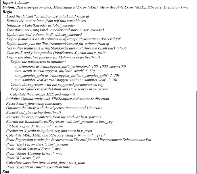
The pseudocode of the proposed hyperopt regression model.
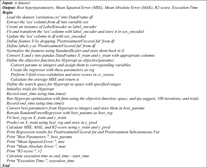
The pseudocode of the proposed hyperopt regression model.
The pseudocode provided outlines two distinct regression processes utilizing a Random Forest Regressor with two different hyperparameter tuning methods: Optuna and Hyperopt. Both algorithms aim to optimize the hyperparameters of the regression model to predict post-treatment visceral fat based on a dataset, and they output the best hyperparameters along with performance metrics such as MSE, MAE, R2-score, and execution time.
Optuna hyperparameter optimization for Random Forest regression
The process begins by loading the dataset ‘cavitation.csv’ into a DataFrame and preparing the data. The ‘sex’ column is extracted, encoded using a LabelEncoder, and updated back into the DataFrame. Features and labels are defined, with features being normalized and both features and labels converted into training DataFrames. An objective function is defined for Optuna, which specifies the hyperparameters to be optimized, such as ‘n_estimators’, ‘max_depth’, ‘min_samples_split’, and ‘min_samples_leaf’. A Random Forest Regressor is created with these parameters, and fivefold cross-validation is performed to calculate the average MSE. An Optuna study is initialized and optimized using the objective function over 100 trials. The best parameters are retrieved, and the RandomForestRegressor is retrained and fitted on the training data. Predictions are made, and performance metrics are calculated and printed, along with the execution time.
Hyperopt hyperparameter optimization for Random Forest regression
Similarly, the Hyperopt process starts by loading the dataset and preparing the data in the same manner as the Optuna process. The objective function for Hyperopt is defined to convert parameters, create the regressor, perform cross-validation, and calculate the average MSE. The search space for Hyperopt is defined with specified ranges for the hyperparameters. Hyperopt optimization is run using the ‘fmin’ function with the objective function, search space, ‘tpe. suggest’, and 100 iterations. The best parameters from Hyperopt are retrieved, and the Random Forest Regressor is retrained and fitted on the training data. Predictions are made, and performance metrics are calculated and printed, along with the execution time.
Both pseudocodes conclude with the printing of regression results for post-treatment visceral and subcutaneous fat, best hyperparameters, MSE, MAE, R2-score, and the execution time. These pseudocodes serve as a step-by-step guide for implementing the proposed regression models with hyperparameter optimization. The following is a pseudocode of the proposed regression process that uses a Random Forest Regressor and Hyperopt for hyperparameter tuning:
Evaluation metrics for regression and classification models
Evaluation metrics for regression models: The determination coefficient R-square is one of the most common performances used to evaluate the regression model as shown in Eq. (1). On the other hand, the Minimum Acceptable Error (MAE) is shown in Eq. (2), while the Mean Square Error (MSE) is investigated in Eq. (3).
$${{\text{R}}}^{2}=\frac{\sum {\left(y-\dot{\widehat{y}}\right)}^{2}}{\sum {\left(y-\dot{\overline{y}}\right)}^{2}}$$
(1)
$${\text{MAE}}=\frac{\sum_{i=1}^{n}\left|\widehat{{y}_{i}}-y\right|}{{\text{n}}}$$
(2)
$${\text{MSE}}=\frac{\sum_{i=1}^{n}{({y}_{i}-\widehat{{y}_{i}})}^{2}}{{\text{n}}}$$
(3)
where y is the actual value, \(\dot{\widehat{{\text{y}}}}\) is the corresponding predicted value, \(\dot{\overline{{\text{y}}}}\) is the mean of the actual values in the set, and n is the total number of test objects41,42,43.
Index of Agreement: Willmott proposed an index of agreement (d) as a standardized measure of the degree of model prediction error which varies between 0 and 1. The index of agreement represents the ratio of the mean square error and the potential error. The agreement value of 1 indicates a perfect match, and 0 indicates no agreement at all. The index of agreement can detect additive and proportional differences in the observed and simulated means and variances; however, d is overly sensitive to extreme values due to the squared differences as shown in Eq. (4)44.
$$d=1-\frac{\sum_{i=1}^{n}{\left({O}_{i}-{P}_{i}\right)}^{2}}{\sum_{i=1}^{n}{\left({|{P}_{i}-\overline{O} }_{i}\left|+{|{O}_{i}-\overline{O} }_{i}\right|\right)}^{2}}, 0\le d\le 1$$
(4)
where Oi is the observation value Pi is the forecast value O bar is the average observation value and P bar is the average forecast value.
Statistical analysis: Posthoc Nemenyi test:
The post hoc Nemenyi test is a multiple comparison test that allows us to compare the pairs of models to determine which pairs are significantly different. The test produces a test statistic called the Nemenyi statistic, which is calculated as in Eq. (5).
$$Nermenyi statistic= {\left(\frac{a}{b}\right)}^{2}{-\left(\frac{c}{d}\right)}^{2}$$
(5)
where a and b are the accuracies of two models being compared, and c and d are the times required to achieve those accuracies. The p-value for the Nemenyi test is calculated as in Eq. (6).
$$p-value = P(Nemenyi \mathrm{statistic }>\mathrm{ observed Nemenyi statistic}) $$
(6)
To determine the best model using statistical analysis, you can perform a post hoc Nemenyi test. The Nemenyi test is a non-parametric statistical test used for multiple comparisons of mean ranks. It can be used to determine if there are significant differences between the models based on the performance measures.
The step-by-step process to perform the posthoc Nemenyi test:
Step 1: Rank the models based on their performance measures. In this case, we can use the mean squared error (MSE), mean absolute error (MAE), and R-squared score.
Step 2: Calculate the average rank for each model across the three performance measures.
Step 3: Calculate the critical difference (CD) value. The CD value represents the minimum difference between the average ranks that is considered significant. It depends on the number of models and the significance level chosen.
Step 4: Compare the average ranks of the models pairwise and check if the difference is greater than the CD value. If the difference is greater, it indicates a significant difference between the models.
Step 5: Based on the results of the pairwise comparisons, identify the best model.
Ethical statement
All procedures performed in studies involving human participants were by the ethical standards of the institutional and/or national research committee and with the 1964 Helsinki Declaration and its later amendments or comparable ethical standards. The study was authorized by the Deraya University Ethical Committee (No: 17/2023). Following a full explanation of the trial, each patient filed a written consent form. The research was carried out at the outpatient clinic from February 2023 to July 30, 2023.
Consent statement
Informed consent was obtained from all individual participants included in the study.