
Ivona Cicovic and Andrea Serafino

Machine learning models are increasingly used in organizational decision-making, but their inner workings remain opaque. If these systems influence real-world outcomes, it’s not enough to know what they predict; you also need to understand why. Explainability techniques aim to reveal this “black box.” Feature attribution tool Those that link predictions to individual inputs are particularly popular. Although it feels intuitive, it relies on strict data assumptions that are rarely true, making the output unreliable. of 2019 Apple Card Case Here’s why this is important. Even though gender is not an explicit input, women appear to receive lower credit limits than men with similar profiles, which is difficult to explain with outcome attribution methods. In this post, we examine the key assumptions underpinning these tools and how they distort their explanations.
Limitations of common explainability methods
Machine learning (ML) models are often so complex that it is difficult to understand how changes in the input data lead to changes in the predictions. This has prompted the development of various explainability techniques that claim to see through this opacity and summarize the relationships between model inputs and outputs.
Common examples include: Shapley Additive Description (SHAP)how to assign each feature an average marginal contribution over all possible feature subsets. Locally Interpretable Model-Independent Explanations (LIME)which explains individual predictions by locally fitting a simple, interpretable model around the observations of interest. Partial Dependency Plot (PDP)a visual tool that shows how a model’s average prediction changes as one feature changes while the influence of other features averages out. and Permuted Feature Importance (PFI)It is a performance-based approach that evaluates feature relevance by randomly shuffling values and measuring the resulting loss in accuracy. However, a growing body of research has highlighted the limitations of these widely used methods, e.g. Salif et al. (2024); Bolt et al. (2022); Velmurugan et al. (2023);and Ragodos et al. (2024)).
A big concern is that these approaches implicitly assume that the model inputs (commonly called features in ML) are independent, an assumption that rarely holds true in real-world datasets. Textbooks and practical guides (e.g. Molnar (2025)) warns about violations of these assumptions, but the warning is often overlooked in real-world applications. While some characteristics of a financial model may be largely independent (for example, number of standing orders and cell phone bill), many other characteristics, such as loan amount and monthly repayments, are naturally correlated. When such dependencies exist, attribution methods produce distorted or misleading explanations, obscuring the true drivers of model behavior. As highlighted in Bank Underground’s previous research on AI fairness, opaque or biased model behavior can both amplify and hide discriminatory decision-making patterns.
Controlled experiments: independent and correlated data
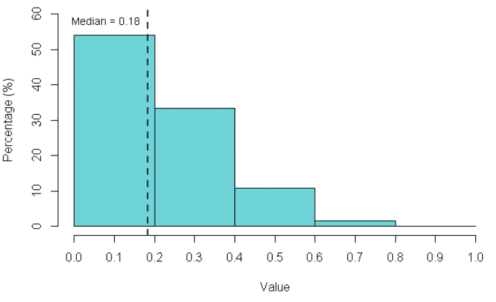
To illustrate how important this is, we perform a simple experiment using two large synthetic data sets (50,000 rows × 50 features). One has independent features (or predictors), and the other has correlated predictors. In both datasets, the target is a linear combination of features and noise. For the correlated feature data set, Chart 1 shows the pairwise correlation heatmap (positive and negative relationships are shown in red and blue, respectively; dark colors indicate strong correlations, light colors indicate weak correlations), and Chart 2 shows the distribution of absolute pairwise correlations. These graphs show patterns typical of many credit risk or economic data sets. Most features have weak relationships, with a median absolute correlation of about 0.20, but a small number of features show stronger associations, closely reflecting those observed, for example, in real-world modeling. Stock and Watson (2017) or Larue et al. (1999)).
For each dataset, we fit four common models: linear regression, random forests, gradient boosting, and neural networks, and applied the four explainability techniques described above. We then compared the feature rankings assigned by these methods to the true rankings implied by the data generation process (i.e., the coefficients used to generate the synthetic data). We measured the rank agreement between the two rankings, i.e., how well the features are arranged in the same order. Spearman’s Rho (ρ) as rank matching coefficient. We repeated this 500 times to see how stable the results were.
Chart 1: Pairwise feature correlation heatmap

Chart 2: Representative distribution of pairwise feature correlations (absolute values)

What the results show
Explainability methods are reliable only when the features are independent, but their performance drops sharply when the features are even slightly correlated (Figure 3). This graph shows the distribution of rank agreement coefficients between estimated and true feature importance rankings over 500 repeated simulation runs. Each panel corresponds to an explainability method and displays a separate boxplot for the model used.
Blue boxplots represent simulations with independent features, and orange boxplots show results when features are correlated. Each box indicates the interquartile range (middle 50% of results), and the median is indicated by a horizontal line. When the features are independent, all methods recover the true rankings with high accuracy and low variability, as reflected in the narrow blue boxplots clustered near 1.
In contrast, ranking performance deteriorates significantly when correlation is introduced. The orange boxplots are much wider, and the median rank agreement coefficient is lower (usually between 0.3 and 0.8), and may even show negative agreement in some runs. This means that truly important features are ranked lower than unimportant features. In real-world settings, typically only a single dataset is observed rather than hundreds of simulations, which means that explaining the importance of a feature by a single model run can be highly misleading. This is of particular concern in high-stakes situations, such as credit scoring, where decisions have real consequences.
Chart 3. Boxplot of rank agreement coefficients between the true feature rankings implied by the data generation process and the rankings implied by different explainability techniques for the top 10 features of a set of models (across 500 simulations).
Chart 3: Boxplot of rank agreement coefficients

To clarify what the coefficients shown in the graph actually mean, it helps to think about what happens in individual model runs. In our simulations, the data generation process is a simple, known linear system, but when features are correlated, explainability techniques often struggle to recover the true order of feature importance.
Two main patterns stand out. First, even truly important predictors can be grossly misrepresented. In many runs, features that are in the top three true drivers of results are pushed far down the rankings produced by explainability techniques, or disappear from the top ten altogether. This shows how easily the actual drivers of model behavior can be obscured when features exhibit even mild dependence.
Second, features that are actually of little or no importance are often promoted to higher ranks. This type of misranking is particularly problematic in practice. This encourages users to build interpretive narratives around variables that played no real role in producing the results, leading to a false understanding of how the model actually works.
Where does this leave us?
In this post, we argue that explainability techniques for feature attribution perform poorly in modern ML environments, where large datasets and interdependent features are the norm. The presented results demonstrate that even modest and realistic levels of feature correlation (on average about 0.20) can significantly reduce the accuracy and stability of common attribution methods. In our simulations, near-perfect rank agreement in the independent setting often drops sharply when correlation is introduced, with important predictors moving down the list and less relevant features moving up. This is important because tools such as SHAP, LIME, PDP, and permutation importance are frequently used to support model interpretation. However, under realistic data conditions, the output becomes less reliable and it becomes difficult to identify which features are truly driving the model’s behavior. If these methods struggle to recover top-level features of clean, fully specified linear systems, serious questions arise about their suitability for describing high-dimensional models used in real-world decision-making. Rather than clarifying the model’s behavior, it reinforces misleading narratives, impedes deeper investigation, risks creating unwarranted confidence, and ultimately sets the stage for bad decisions.
For feature attribution to be truly insightful, it requires much more structure than most ML pipelines support. That means implementing disciplined feature construction: explicitly mapping correlation structures, grouping variables into interpretable clusters (e.g., socio-economic status, credit trends, stability, demographics), and reporting explanations at the group level rather than individual features.
While this kind of structured organization is standard in classical statistics, many modern ML pipelines instead rely on large sets of raw or automatically engineered features. In such settings, models are often trained on whatever variables are available in the dataset in hopes that the learning algorithm will discover useful structure without extensive manual grouping by domain. As a result, explicit feature grouping is rarely incorporated into modern ML workflows, and with many correlated variables, defining meaningful groups can become a research task in itself.
It is worth noting that there are imputation techniques designed to relax the independence assumption. conditional SHAP and causal SHAP – But these are very difficult to scale. Conditional SHAP requires estimating the joint feature distribution to compute the conditional expectation. Causal SHAP requires a well-specified causal graph, which most practical ML projects lack. Both are very computationally expensive and fragile in high dimensions. Therefore, although these alternatives address some of the theoretical shortcomings of classical feature attribution methods, they are still largely impractical for everyday ML use. This leaves a significant gap between what explainability methods promise in principle and what they can realistically deliver today.
These findings demonstrate that we need to rethink how we evaluate ML models, rather than treating feature attribution as the primary means of understanding the model. One way to move beyond attribution is to examine model behavior by examining how the output changes under structured “assumptions” changes in the input. A detailed explanation of this and other approaches is beyond the scope of this post.
Ivona Cickovic and Andrea Serafino work in the Bank’s Model Review and Development department.
If you would like to contact us, please send an email to the address below. Bankunderground@bankofengland.co.uk Or leave a comment below.
comment It will only be displayed if approved by a moderator and will only be published if your full name is provided. Bank Underground is a blog where Bank of England staff share views that challenge or support prevailing policy wisdom. The views expressed here are those of the authors and not necessarily those of the Bank of England or its Policy Committee.
Share the post “Machine Learning Explainability: Do Common Techniques Deliver Their Promise?”


