The method of GCW optimization can generally be divided into three main steps (Fig. 1). The first step is numerical simulation, in which datasets for machine learning are obtained. The second step is machine learning, in which the acquired datasets are used to train the models for optimizing the parameters of GCW. In this research, Multiple Linear Regression (MLR), Artificial Neural Networks (ANN), and Support Vector Machine (SVM) were applied to train and appraise the optimization models. In the third step, the parameters of the GCW are optimized for the test site.

Framework of GCW optimization.
Confirmation of characterization indicators and influence factors
-
1.
Indicators of circulation efficiency: Typically, the flow field induced by GCW exhibits the traits depicted in Fig. 2. It can be segmented into three parts, the upstream capture zone, the circulation zone, and the downstream release zone 7. In order to characterize of groundwater features surround the GCW, two indicators are usually applied8,13,16: the radius of influence (R) and the particle recovery ratio (Pr).
Figure 2 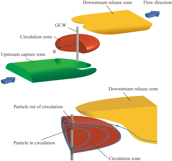
Indicators of GCW operation efficiency.
-
①
Radius of influence (R): The variable R plays a crucial role in defining the range of influence within the circulation zone. This represented the greatest horizontal separation from the circulation zone’s edge to the axis of the well. The hydraulic gradient alters the form of the circulation area, leading to fluctuating R values in different orientations. Therefore, there is a variance in the radius both along and at right angles to the groundwater flow. The indicator R, identified as the upstream radius parallel to the hydraulic gradient, is ascertainable through the computation of the distance between the particle migration trajectory in the particle tracking model.
-
②
Particle recovery (Pr): The variable Pr serves as a measure for the groundwater’s capacity to be captured by the extraction screen. Groundwater from the injection screen moves towards two areas: the extraction screens and the downstream release zone. To quantify the indicator via numerical simulation, the results of particle tracking were calculated by MODPATH12,17. The value of Pr can be expressed as the proportion of particles in the circulation zone to the total number (Ncycle/Ntotal). The schematic diagram of the indicators is shown in Fig. 3.
Figure 3 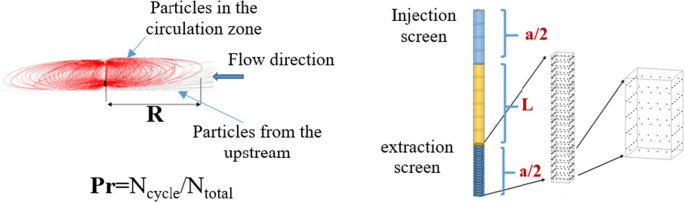
The schematic diagram of the indicators.
-
①


-
2.
Influence factors: The success of GCW operations largely stems forms the hydrogeological conditions of the remediation site. In addition, the configuration and operation mode of GCW are also crucial8,28. This study focused on identifying key factors influencing of GCW’s operations and their corresponding indicators of characterization. The key elements are listed below.
-
①
Hydrogeological parameters: Typically, hydrogeological parameters are employed to assess the appropriateness of the GCW techniques. This research primarily focused on defining hydrogeological parameters such as the horizontal conductivity (KH), vertical hydraulic conductivity (KV), the vertical heterogeneity (KH/KV), aquifer thickness (M), porosity (n), specific yield (μ), and hydraulic gradient (I).
-
②
Structure and operation parameters: The distance between the top of the upper screen section and the bottom of the lower screen section (L) and the total length of the two screen sections (a) were used as the indicators of the circulation well structure parameters; the pumping rate (Q) was used as the main indicator of operating parameters12,16.
-
①
Development of database for machine learning
The machine learning database was developed utilizing the FloPy package in conjunction with Python. A variety of tools exist for developing models, encompassing Python-based packages for plotting, manipulating arrays, optimizing, and analyzing data. In particular, FloPy was chosen for creating GCW numerical models due to its adaptability in handling MODFLOW and MODPATH packages via coding29. By entering varied parameter values, we derived diverse characterization indicators for GCW, leading to the creation of a database. Ultimately, the FloPy program efficiently produced over 3000 samples suitable for machine learning applications. An in-depth account of how the database was developed is provided in the supplementary material.
Machine learning approaches
According to the views of formal researchers and the preliminary work of this study30,31, the key indicators R and Pr were designed as the output variables. The influence variables M, Q, I, μ, n, a, and L were set as the input variables. A reliable and effective database is important to the performance and the conclusion of machine learning. So, data cleaning before training plays a crucial role in the realm of machine learning. Box plots were used to eliminate abnormal values, and NaN (not a number), rather than numerical ones, were removed. Following the cleaning of data, the database was divided randomly into two groups; after several trials, the model results were found to be optimal for 80% and 20% of the data assigned to the training and test sets, respectively. Utilizing the training dataset, the model was trained to derive the functions linking the input and output variables. The test dataset was applied to assess the model’s forecasting capabilities.
Database preprocessing
The application of computer technology to imitate human learning activities is a relatively new field of research18,32. A variety of analytical techniques are utilized within machine learning algorithms to construct related models. Each of these models is employed to deduce new tasks form the data.
Generally, machine learning algorithms can be categorized into two types based on their modeling methods: supervised and unsupervised learning. Supervised learning involves training a model to elucidate the link between feature variables and their results. Conversely, in the realm into the unexplored configurations of a specific given dataset33. The aim of this research was to explore how characterization indicators correlate with influence factors. It is a typical regression problem. Consequently, the method involving partially supervised learning method was applied. MLR, ANN, and SVM serve as effective techniques in addressing regression issues.
Model training
Python, known for its readability, interactivity, and cross-platform nature, excels in code development efficiency. Scikit-learn is a package of Python that integrates a variety of advanced machine learning algorithms and can be used to solve medium-scale supervised and unsupervised problems34,35. In this research, three distinct algorithms (MLR, ANN, SVM) for model training within the Scikit-learn package were adopted. The theory of the algorithms are as follows.
-
1.
Multiple linear regression
Multiple linear regression (MLR) is the most common method for determining the linear relationship between input and output variables when handling features with limited data. The MLR method was applied to find a linear correlation between input and output variables. The mathematical form is as follows25:
$$ \hat{y} = b_{1} x_{1} + b_{2} x_{2} + \cdots + b_{n} x_{n} + c $$
(1)
where \(\hat{y}\) is the regressor; \(b_{i}\) (i = 0, 1, 2, …, n) is the coefficient of each variable, which represents the weight of the variable;\(x_{i}\)(i = 1, 2, …, n) is the input variable of the regression; c is the intercept term. Through continuous training, the values of bi and c are confirmed according to the minimization of the fitting error between the forecasted and actual value. The key of MLR method is the least squares method which is widely employed to estimate the parameters by fitting a function to a set of measured data. This approach seeks to identify the best outcome when the sum of squares error (SSE) is minimized. SSE can be defined as follows:
$$ SSE = \sum\nolimits_{1}^{n} {r_{i}^{2} } $$
(2)
where
$$ r_{i} = y_{i} – f(x_{i} ,\beta_{i} ) $$
(3)
SSE values approaching zero indicate the closeness of estimated parameters to the actual value. If \(f(x_{i} ,\beta_{i} )\) is linear, then it is a linear least square. The least squares model can be solved by employing simple calculus. However, if \(f(x_{i} ,\beta_{i} )\) is nonlinear, it can be solved by an iterative numerical approach 30.
-
2.
Artificial neural networks
Artificial neural networks (ANN) can execute learning and prediction functions through the emulation of human learning processes. ANN is capable of identifying links between input and output data while forming and fortifying neurons connections26,36. An algorithm based on a multi-layer perception neural network could rank as the top choice among artificial neural network algorithms. Due to its capability to tackle complex regression problems, this research opted to develop artificial neural networks featuring input, output, and hidden layers to enhance GCW optimization (Fig. 4).

Structure of ANN for optimization of GCW.
Neurons linked in unison convert the input data into output values. In the input layer, seven neurons, symbolizing seven input variables, were established. A single neuron, symbolizing an individual goal for each predictive issue, was set in the output layer. Numerous experiments were conducted to ascertain the optimal hyper-parameters. To forecast R and Pr, four hidden layers were set, starting with 256 neurons, followed by 128 neurons in the next layer, 64 neurons in the third, and 32 neurons in the fourth. The design of the model can be described as follows:
$$ {\text{x}}_{t + T}^{F} = F(X_{t} ,w,\theta ,m,h) = \theta_{0} + \sum\limits_{j = 1}^{h} {w_{j}^{out} } f\left( {\sum\limits_{i = 1}^{m} {w_{ji} x_{t – i + 1} + \theta_{j} } } \right) $$
(4)
where \({\text{x}}_{t – i + 1} ,i = 1,…,m\) represents the element of the input vector \(X_{t}\); \({\text{w}}_{ji}\) is the weight determining the relationship between the nodes; \(\theta_{0}\) is the bias of the output node; \(f( \cdot )\) is the transfer function. Following extensive experimentation, the optimal hyper-parameter was ascertained. The Rectified Linear Unit (ReLU) serves as the ideal transfer function for forecasting R (Eq. 5). Yet, in predicting Pr, tanh (Eq. 6) ought to serve as the optimal transfer function. By utilizing neural networks, the value of loss progressively diminishes and reaches stability following 110 interactions. Consequently, the maximum number of iterations that yield reliable predictive outcomes for models ought to be 110.
$$ f(x) = \max (x,0) $$
(5)
$$ y = \tanh (x) = \frac{{e^{x} – e^{ – x} }}{{e^{x} + e^{ – x} }} $$
(6)
-
3.
Support vector machines
The Support Vector Machines (SVM) employs the kernel functions to convert the data into a hyperspace, enabling the representation of intricate patterns36,37,38,39. With the emerging hyperspace, SVMs aim to develop a hyperplane suitable for categorizing and constructing the broadest data margin, or one that accommodates data with minimal complexity and reduced empirical risk associated with the modelling function27. SVMs have been applied recently for many purposes in the field of hydrogeology40,41,42. In this study, the training data can be presented as {(xi, yi), i = 1, 2,3, …, n}, where x is the input variable, and y is the output variable. A loss function offered by the SVM can be delineated in the following manner43,44,45:
$$ L_{\varepsilon } (y,f(x,\omega )) = \left\{ \begin{gathered} \, 0 \quad if\left| {y – (\omega \phi {(}x{) + }b)} \right| \le \varepsilon \hfill \\ \left| {y – (\omega \phi (x){ + }b)} \right| – \varepsilon \quad otherwise \hfill \\ \end{gathered} \right. $$
(7)
The issue with SVM can be characterized as the following optimization problem:
$$ {\text{minimize}}\;\;R_{{\omega ,\xi_{i}^{{}} ,\xi_{i}^{*} }} = \frac{1}{2}\left\| {\left. \omega \right\|} \right.^{2} + C\sum\limits_{i = 1}^{n} {\left( {\xi_{i}^{{}} + \xi_{i}^{*} } \right)} $$
(8)
$$ {\text{subject to}}\;\;\left\{ \begin{gathered} {\text{y}}_{{\text{i}}} – f(\phi (x_{i} ),\omega ) – b \le \varepsilon + \xi_{i}^{{}} \hfill \\ f(\phi (x_{i} ),\omega ) + b – y_{i} \le \varepsilon + \xi_{i}^{*} \hfill \\ \xi_{i}^{{}} ,\xi_{i}^{*} \ge 0 \hfill \\ \end{gathered} \right. $$
(9)
where \(\phi \left( x \right)\) is a kernel function designed for projecting the data into a hyperspace; \(\frac{1}{2}\left\| \omega \right\|^{2}\) stands for generalization; \(C\mathop \sum \limits_{i = 1}^{n} \left( {\xi_{i} + \xi_{i}^{*} } \right)\) represents empirical risk; \(\xi_{i}\) and \(\xi_{i}^{*}\) are slack variables for measuring “below” and “above” the \(\varepsilon\) tube (Fig. 5). Slack variables hold positive values while \(C\) remains a positive constant.

Support vector regression.
Model testing and comparison
The testing dataset was used to test the MLR, SVM, and ANN models by comparing their performance with statistical measures. The precision was evaluated by computing the coefficient of determination (R2) and Root Mean Square Error (RMSE) using the fitting curve. A near-1 absolute value of R2 suggests enhanced precision within the model. When the RMSE value nears 0, there is an enhancement in the model’s fit. Their mathematical formulas are as follows:
$$ R^{2} = \frac{{\sum\limits_{i = 1}^{n} {(\hat{y}_{i} – \overline{y})} }}{{\sum\limits_{i = 1}^{n} {(y_{i} – \overline{y})^{2} } }} $$
(10)
$$ RMSE = \sqrt {\frac{1}{n}\sum\limits_{i = 1}^{n} {(\hat{y}_{i} – y_{i} )^{2} } } $$
(11)
where \(\hat{y}_{i}\) is the estimated value; \(y_{i}\) is the actual value; n is the number of actual values.