Deep-learning deconvolution and segmentation of fluorescent membranes for high-precision bacterial cell-size profiling

Strains and plasmids

A list of strains is provided in Supplementary Table 1. Plasmid and primer lists are in Supplementary Tables 2 and 3, along with detailed descriptions of plasmid construction.

Culture media and growth conditions

Bacteria were routinely grown on LB agar plates (Lennox formulation, 5 g NaCl/L) overnight at 30 °C, with the exception of Lactococcus lactis, which was grown on MRS medium at 28 °C. Saccharomyces cerevisiae was grown on YPD at 37 °C.

For size quantification of B. subtilis and P. megaterium strains, a single colony was inoculated into 5 mL fresh LB Lennox and grown overnight in a roller drum at 30 °C with constant rotation. The next morning, cultures were diluted 1:1000 into 30 mL of the appropriate medium in 250-mL baffled flasks and incubated in a water bath at 30 °C with shaking at 220 rpm. Samples were taken after five hours (exponential; Supplementary Fig. 10) and after ten hours (stationary; Supplementary Fig. 10) for microscopy (see next section).

For the induction experiments shown in Fig. 6 and Supplementary Fig. 14, a single colony was inoculated into LB Lennox diluted 1/4, then grown at 25 °C in a shaking incubator at 220 rpm. The next morning, cultures were diluted to an OD600 of 0.02 in 1/4-diluted LB Lennox with the indicated IPTG concentration (0, 25, 50, 100, 500, or 1000 µM). Cultures were grown at 30 °C in a shaking incubator to an OD600 of 0.2–0.5 and then samples were taken for microscopy.

Sporulation (Fig. 4e) was induced by resuspension, as described elsewhere⁸⁷.

Microscopy

For imaging, 10 µL culture samples were imaged on 1.2% agarose pads in 1/4-diluted LB-Lennox supplemented with 0.5 µg/mL FM4-64. The pad was covered with a #1.5 glass coverslip. Ten-hour samples were diluted three times to avoid overcrowded fields.

For cell-size estimation experiments for the different B. subtilis and P. megaterium strains, cells were imaged using a Leica Thunder Imager live cell with a Leica DFC9000 GTC sCMOS camera and a 100X HC PL APO objective (Numerical aperture 1.4, Refractive index 1.518 objective). FM 4-64 images were taken using a 510 nm excitation LED light source, with 70% intensity and 0.1 s exposure, and a custom filter cube produced by Chroma Technology GmbH (Olching, Germany) with the following components: excitation filter, ET505/20x; dichroic mirror, T660lpxr; emission filter, ET700lp. Training images for the restoration (FM2FM and FM2FM-HiSNR) and translation (FP2FM) models were taken with a DeltaVision Ultra microscope with a PCO Edge sCMOS camera and an Olympus 100X UPLX APO objective (Numerical aperture 1.45, Refractive index 1.518 Ph3). FM 4-64 and mVenusQ69M were visualized with the following filters: excitation 542 nm and emission 679 nm for FM 4-64, and excitation 475 nm and emission 525 nm for mVenusQ69M, with light transmission at 100% and an exposure time of 0.2 s for both channels. Training images for the segmentation models (FMSeg, RawFMSeg) were taken using the same illumination conditions as the restoration model. For the membrane images of E. coli, the FM4-64 was captured with light transmission of 40% and an exposure time of 0.1 s.

For phase-contrast microscopy, the aforementioned DeltaVision microscope was used, with light transmission set to 100% and exposure time to 0.1s.

For microscopy comparisons, we also used a Zeiss Axio Imager Z2 microscope with a Hamamatsu sCMOS camera and a Zeiss 100x Plan-Apochromat objective (Numerical aperture 1.40, Refractive index 1.518 Ph3). FM 4-64 was visualized with an excitation filter of 506 nm and emission filter of 751 nm, with light transmission at 100% and an exposure time of 0.2 s.

Ground truth image annotation using active contours

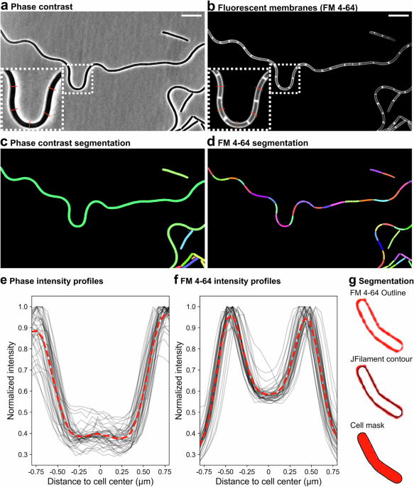
We annotated cells in our ground-truth images using the ImageJ plugin JFilament³⁶, which allows the semi-automatic generation of sub-pixel resolution active contours (snakes) that follow the ridges of maximum fluorescence membrane intensity around the cell (Fig. 1f; Supplementary Fig. 1)^3,71,88. Default parameters were used, except for Gamma, which we increased when the preset value led to excessive snake deformation. For cell clusters, snakes were typically manually corrected because contour edges tended to deform toward neighboring cells. When membrane blobs distorted cell contours, we also corrected the snakes to follow straight lines. These steps ensured consistent single-cell segmentation during model training and improved the segmentation model’s robustness to such confounding artifacts.

Training and evaluation of models for segmenting fluorescent membranes

We annotated 143 raw and SoftWorx (Cytiva Life Sciences)-deconvolved FM 4-64 membrane images using JFilament³⁶, as described above, yielding over 7000 cells for training. Training images were maximum-intensity projections of FM4-64 z-stacks. Following the Omnipose documentation¹⁴, we trained the models from scratch, i.e., not using any existing model parameters as starting points. In contrast, for Cellpose3³⁵, Cellpose-SAM²¹ and microSAM²⁰, the existing base models were fine-tuned with the existing data. All trainings were done following the suggestions found in their respective documentation. Omnipose models were trained with a batch size of 8 images for 4000 epochs using a learning rate of 0.1 and a Rectified Adam (RAdam) optimizer⁸⁹. Both models (raw and deconvolved) were trained using the same parameters. Cellpose3 models were trained with a batch size of 1 image for 100 epochs using a learning rate of 0.1, a weight decay of 1×10^-4, and a Stochastic Gradient Descent (SGD) optimizer⁹⁰. Both models (raw and deconvolved) were trained using the same parameters. Cellpose-SAM models were trained with a batch size of 1 image for 100 epochs using a learning rate of 1×10^-5, a weight decay of 0.1, a tile size of 256×256 px, and an AdamW optimizer⁹¹. Both models (raw and deconvolved) were trained using the same parameters. MicroSAM models were trained with a batch size of 1 image for 10 epochs of 1788 iterations per epoch, using a learning rate of 1×10^-5, a weight decay of 0.1, a tile size of 512×512 px, and an AdamW optimizer. Segmentation decoder was also trained to allow for automatic instance segmentation. Both models (raw and deconvolved) were trained using the same parameters.

Training was done in the “deepbio” computing cluster at the Max Planck Institute for Evolutionary Biology, using a single NVIDIA(R) GeForce GTX 2080 Ti GPU with 12GB memory.

For accuracy assessment, we annotated 56 images with JFilament. F1 score^92,93,94 was calculated at eleven Intersection over Union (IoU) thresholds spanning 0.5 to 1, in 0.05 intervals. True positives, false positives, and false negatives were calculated using the Omnipose library function “average_precision”. F1 was then computed using these values following Caicedo et al. 2019⁹².

Simulation of fluorescent membranes

Synthetic rod-shaped cells were generated using SyMBac⁹⁵, with a constant length of 4 µm and variable widths, at a pixel size of 15 nm. Contours were extracted from each plane of each synthetic cell to represent the membrane. To simulate membrane staining, 90% of contour points were randomly selected for the placement of fluorescence molecules. To model light spread, a synthetic point spread function was generated in SyMBac using the “3 d fluo” mode with the following parameters: radius = 150, wavelength = 600 nm, numerical aperture = 1.49, refractive index = 1.5, and pixel size = 15 nm. To measure cell width from JFilament-generated masks (Supplementary Fig. 1), simulated images were rescaled to a pixel size of 65 nm to match our microscopy images. Measurements were performed on the middle focal plane of the simulated z-stacks.

Training and evaluation of models for deconvolution prediction (FM2FM) and fluorescence translation (FP2FM)

Deconvolution-prediction and fluorescence-translation models were trained using the Content Aware Restoration (CARE) framework⁴⁰. For FM2FM and FP2FM model, 200 images (2048×2048 pixels) of vegetatively growing B. subtilis constitutively expressing mVenusQ69M⁹⁶ were acquired using a DeltaVision Ultra microscope with a PCO Edge sCMOS camera, capturing FM4-64 membrane fluorescence, and mVenusQ69M cytoplasmic fluorescence. Images were deconvolved in the DeltaVision software (SoftWorx) and then cropped to remove deconvolution edge artifacts, yielding 1914×1914 px image outputs. Non-deconvolved training inputs were cropped to the same size. Training input images were single-plane images of raw FM4-64 (for the FM2FM model) or mVenusQ69M (for the FP2FM model) z-stacks, and target images were the deconvolved FM4-64 images for both models. For training, 16 patches of 512×512 px were extracted from each image pair. Models were then trained using a batch size of 32 images for 100 epochs, with 100 training steps per epoch. Training was performed in the “deepbio” computing cluster at the Max Planck Institute for Evolutionary Biology, as above. Model parameters and training hardware was the same for both models.

To compare model performance against the membrane deconvolution target (SoftWorx), we conducted qualitative assessments of output images’ intensity profiles. We quantified the Structural Similarity Index Measure (SSIM) between the extracted image patches. Patches were selected to maximize the number of cells and minimize the background. SSIM was calculated using the Python scikit-image library⁹⁷. We then statistically compared cell-size estimates using membrane images deconvolved with SoftWorx or predicted with FM2FM or FP2FM (Fig. 3; Supplementary Fig. 6). Width, Length, Surface Area, and Volume were measured using the skeletons as explained further down. Cross-sectional area, convex hull area, eccentricity, and solidity, were directly obtained from segmentation masks using the Python scikit-image library⁹⁷.

Training and evaluation of a deconvolution-prediction model that increases the signal-to-noise ratio (SNR) of predicted images (FM2FM-HiSNR)

We use CARE⁴⁰ to train an additional deconvolution prediction model that produces high signal-to-noise ratio (SNR) images from low-SNR non-deconvolved fluorescent membrane images. We named the model FM2FM-HiSNR. FM 4-64 images of vegetatively growing B. subtilis were acquired at four different illumination conditions using a DeltaVision Ultra microscope with a PCO Edge sCMOS camera. The illumination conditions were as follows (exposure time and percentage of transmitted light listed after their names in quotation marks): “Noisy”, 0.01 s, 10%; “i1”, 0.01 s, 50%; “i2”, 0.025 s, 10%; “Target”, 0.2 s, 100%. Images were deconvolved using the DeltaVision software (SoftWorx) and then cropped to remove deconvolution edge artifacts, yielding 1914×1914 px image outputs. Non-deconvolved training inputs were cropped to the same size. Training input images were single-plane images of raw FM4-64 z-stacks from all different illumination conditions, and target images were the deconvolved FM4-64 images at the “Target” illumination condition. In total, 98 input images were used. For training, 16 patches of 512×512 px were extracted from each image pair. The model was then trained using a batch size of 32 images for 100 epochs, with 100 training steps per epoch. Training was performed in the “deepbio” computing cluster at the Max Planck Institute for Evolutionary Biology, as above.

To explore the relationship between SNR and segmentation accuracy, and to test whether restoration with FM2FM-HiSNR improve segmentation accuracy of low SNR images, FM 4-64 images of vegetatively growing B. subtilis were acquired at 12 different illumination conditions using a DeltaVision Ultra microscope, under the following illumination conditions (exposure time and percentage of transmitted light listed after their names in quotation marks): “Noisy”, 0.01 s, 10%; “i1”, 0.01 s, 50%; “i2”, 0.025 s, 10%; “i3”, 0.025 s, 50%; “i4”, 0.05 s, 10%; “i5”, 0.05 s, 50%; “i6”, 0.1 s, 10%; “i7”, 0.1 s, 50%; “i8”, 0.1 s, 100%; “i9”, 0.2 s, 10%; “i10”, 0.2 s, 50%; “Target”, 0.2 s, 100%. Images were deconvolved using the DeltaVision software (SoftWorx) or restored with FM2FM-HiSNR, and segmentation accuracy was calculated (Supplementary Fig. 13).

Extracting cell size information from masks of rod-shaped cells

For rod-shaped bacteria, we assumed a sphero-cylindrical geometry with hemispherical caps⁵⁶. First, we computed the minimum Euclidean distance from each pixel inside the mask to the closest pixel on the mask boundary⁹⁸, which is commonly referred to as the distance transform. Next, we generated a one-dimensional centerline (commonly known as “skeleton”)⁹⁹, overlaid it on the distance transform map, and determined the distance value at each skeleton pixel, thereby obtaining the local radius of the mask along the skeleton line (Fig. 4a). An alternative one-dimensional representation is the medial axis¹⁰⁰, also known as the “topological skeleton” (Supplementary Fig. 15). We compared size estimates obtained with the two representations and found significant differences in some size metrics in a set of E. coli cells (Supplementary Fig. 15d). Inspection of individual masks revealed that some medial-axis representations tended to over-branch (Supplementary Fig. 15e). If common across many cells, such over-branching would lead to inaccurate size estimates. We therefore proceeded with the skeleton representation.

To estimate the extent of the hemispherical caps, we took the distance between each skeleton endpoint and the corresponding mask tip as the cell radius at the skeleton endpoints. This yielded precise estimates of mask length, and with profiles at every pixel along the skeleton. Assuming rotational symmetry and that the masks derive from medial focal-plane images, we estimated cell volume and surface area by adding the volumes and lateral surface areas of cylindrical segments generated by circularly projecting the radius of the mask at each pixel of the skeleton, plus the hemispherical caps (Fig. 4a). This approach accurately handles elongated masks, provides local morphological information of cell morphology, and is robust to cellular curvature. While tailored to rods, the framework can be adapted to other morphologies.

Dealing with branching skeletons

Due to the mask geometry, it is possible that the skeleton branches into multiple endpoints (Supplementary Fig. 15c). To handle both branched and non-branched cases, we developed the following workflow. First, we treat the skeleton as a graph, with each pixel considered a node. Assuming connectivity only between neighboring pixels (horizontal, vertical, or diagonal), we define edges for pairs of pixels whose Euclidean distance is less than 1.5 pixels, thereby retaining connected neighbors. Next, we implement a Depth-first search (DFS) algorithm to find the longest possible path connecting the opposite endpoints in the graph. If the skeleton is not branched, this path corresponds to the skeleton. For branched skeletons, multiple candidate paths exist. For each candidate path, we compute the cell size metrics described in the next section and take the median of each metric as the cell size (Supplementary Fig. 15).

Cell size measurements

We combined the mask skeleton and distance transform to derive cell measurements under a spherocylindrical geometry with hemispherical caps and rotational symmetry. The measurements are implemented in a custom code written in Python3, which can be found in the GitHub repository linked in the “Code availability” section.

Cell length (L) is the sum of Euclidean distances d between two successive points in the mask skeleton, plus the distance from each skeleton endpoint and the corresponding mask tip, which corresponds to the local radius at the skeleton endpoint r_s. With that, L follows the equation:

Cell width (w_i) is calculated as twice the value of the radius at each point in the skeleton (r_c). Mean w can then be calculated as:

Cell surface area (S) is calculated as the sum of lateral surface areas of the cylinders projected at each point in the skeleton, with radius r_c and height h of 1 pixel, plus the lateral surface area of the hemispherical caps with radius r_s. Thus, S is calculated as:

Cell volume (V) is obtained similarly to S, as it adds the volume of each cylinder and the hemispherical caps (with same parameters of radius and height as S). V is then obtained from:

Measurement transformation

We segmented 864 single cells of Escherichia coli stained with FM 4-64 using either JFilament (ground-truth) or FMseg. Cells were from early exponential phase (OD₆₀₀ = 0.1-0.3) cultures in either LB Lennox, or MOPS minimal medium with 0.1% glucose, providing a range of cell widths from 0.53 to 1.04 µm, and a range of cell lengths from 0.87 to 9.61 µm (based on measurements from ground-truth masks) (Supplementary Fig 8a). Measurements from ground-truth masks were plotted against the values obtained from on the FMseg-generated masks, revealing a consistent size overestimation for FMseg masks (Supplementary Fig. 8b). The data show a linear relationship for the overestimation, which allows us to leverage statistical tools to compute the necessary parameters to transform the data between the automatic segmentation results and the ground truth results. A linear regression would be a direct way to do this, extracting the values for the slope (m) and intercept (n) necessary to transform the data. While linear regression returns a coefficient of error that would allow us to simulate distributions to sample m and n, there is the chance that we may over- or under-estimate these values, as well as sample pairs that do not make sense in the context of our data. Thus, we leveraged the PYMC library¹⁰¹ and its use of Bayesian statistics for sampling the necessary parameters, which are m, the fit slope, n, the fit intercept, and σ, the standard deviation of our sampled observations. Since our data behaves linearly, we used a Bayesian Generalized Linear Model (GLM), assuming that our parameters (slope, intercept, size metric, and its standard deviation) follow certain types of distributions. For σ, we assume a Half-Cauchy distribution, which only returns positive, non-zero values, which is the only type of values a standard deviation can have. For m and n, we sample from normal distributions with mean 0 and standard deviation 20, giving us a wide range of possible parameters. Then, for computing the observed values, we also assume a normal distribution. PYMC performs a series of draws to fit the data and thus after successive draws we end with the distributions of m, n and σ. In our case, we performed four chains of 3000 draws each, giving us a total of 12000 sampled values. We can then randomly sample pairs from these distributions in order to transform the data, as well as to include the uncertainty of the transformation in the analysis (Supplementary Fig. 8b). For the examples shown in Fig. 5, Fig. 6, and Supplementary Fig. 11, we sampled 250 pairs of m and n for each individual cell measurement, thus allowing us to compute new metrics.

Statistics and reproducibility

For the statistical tests in Fig. 3, Fig. 6, Supplementary Fig. 6, and Supplementary Fig. 15, Levene’s test was computed for the distributions of interest. If the p-value was greater than 0.05, one-way ANOVA was performed to obtain the p-values and determine if the difference between distributions was significant or not. In cases where Levene’s test was significant (p < 0.05), Kruskal test was used instead. All three tests were used as they are implemented in SciPy¹⁰². Each individual cell was considered as a replicate for the purposes of the statistical tests. Sample sizes are specified either in the figure legends or inset in the plots.

CryoEM image analysis

Because the high magnification of the cryo-EM images typically did not capture entire cells, we estimated cell width as the straight-line distance between the mother-cell lateral membranes, measured perpendicular to the cell longitudinal axis. In cryo-FIB tomograms of wild-type cells, only a portion of the cellular volume was retained: focused ion-beam milling produced a thin lamella that sampled a section of the cell. We analyzed only tomograms in which this section included the mid-cell region. To verify this, we measured width across successive z-slices and selected tomograms showing a clear width peak at mid-cell that decreased in slices above and below.

Whole genome sequencing

For whole-genome sequencing, Priestia megaterium WH320 was streaked in an LB-Lennox agar plate and grown overnight at 30°C. Next morning, a single colony was picked and re-streaked in an LB-Lennox agar plate and grown overnight at 30°C. Cells were collected from the plate and genomic DNA was extracted with the MasterPure Gram Positive DNA Purification Kit (Biosearch technologies). Extracted genome was then sequenced using an Illumina NextSeq 500 sequencer. Raw pair-end sequences were loaded into Geneious prime version 2025.1.2 for sequence trimming and pairing with an insert size of 500 base pairs. Paired sequence list was then exported in fastq format for analysis using breseq¹⁰³.

Software and data availability

The fine-tuned segmentation models for raw and deconvolved images (for Omnipose, Cellpose-SAM, microSAM, and Cellpose3), deconvolution prediction (FM2FM), deconvolution prediction and SNR increase (FM2FM-HiSNR2), and fluorescence translation (FP2FM) models can be found in the Zenodo (https://zenodo.org/records/18978187). Segmentation model training and benchmarking data can be found at the BioImage Archive repository https://www.ebi.ac.uk/biostudies/studies/S-BIAD2350. Deconvolution model training and benchmarking data can be found at the BioImage Archive repository https://www.ebi.ac.uk/biostudies/studies/S-BIAD2353. Images of individual E. coli cells used for measurement transformation with their corresponding annotations and automatic segmentations be found at the BioImage Archive repository https://www.ebi.ac.uk/biostudies/studies/S-BIAD2352. Segmentation of B. subtilis and P. megaterium strains (wild-type and induction constructs) be found at the BioImage Archive repository https://www.ebi.ac.uk/biostudies/studies/S-BIAD2354. P. megaterium WH320 genome sequence has been deposited in ENA (accession number PRJEB112284). PBP 1 A/1B protein sequence alignment, and results from breseq¹⁰³ are available in Zenodo¹⁰⁴. Raw data files for reproducing the plots are available in Zenodo¹⁰⁵. All other data are available from the corresponding author on reasonable request.