Data Sources and Preprocessing
The dataset used in this study was obtained as lateral thoracic-lumbar radiographs of patients from Ansan Hospital, a university in South Korea. The collected dataset included 487 radiographs with fractures and 141 normal radiographs. Only radiographs that were confirmed as compression fractures based on MRI results were collected and labeled. The radiographs were anonymized before use, and each patient's personal information was removed in accordance with ethical guidelines. Overall, 598 segmentation masks of marked fractures were extracted from the 487 lateral thoracic-lumbar radiographs and used to train and test each model.
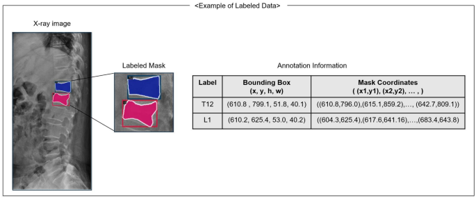
A total of six MRI-based class labels were defined and their locations were marked during data preprocessing: L1, L2, L3, L4, T11, and T12 fractures. Two orthopedic experts labeled the vertebrae location and type using the open source labeling software “labelme” version 5.0.2 (https://github.com/labelmeai/labelme).16Each polygon mask contains fracture information for six classes (L1-T11) and the coordinates of the fractures identified at each point of the polygon. Figure 1 shows an example of the labeled data used in training. In approximately 20% of patients, multiple VCFs were identified and labeled as separate polygons.

Example of labeled data. Each fracture is labeled with a polygon on a thoracic-lumbar spine radiograph based on the MRI results. Each polygon mask contains the x and y coordinates of the polygon mask that encloses it. Each bounding box consists of the top-left x and y coordinates, width, and height. The entire labeling process was performed by two trained orthopedic experts.
Study setting
In this study, about 70% of the dataset (346 radiographs) was used to train the neural network, and about 15% was allocated to validation data (71 radiographs) and test data (70 radiographs), respectively. The training, validation, and test data were split in a hierarchical manner to take into account the class-wise distribution. Radiographs without fractures were only used in the testing phase. Stochastic gradient descent with momentum was used as the optimization technique. The learning rate was set to decrease with a weight decay of 0.0001 and momentum of 0.9. Transfer learning was used.17 To improve model performance, each model was trained from pre-trained weights on the COCO instance segmentation dataset.18A horizontal flip and a 10 degree random rotation extension were applied. An overview of the VCF dataset is shown in Table 1.
Mask R-CNN
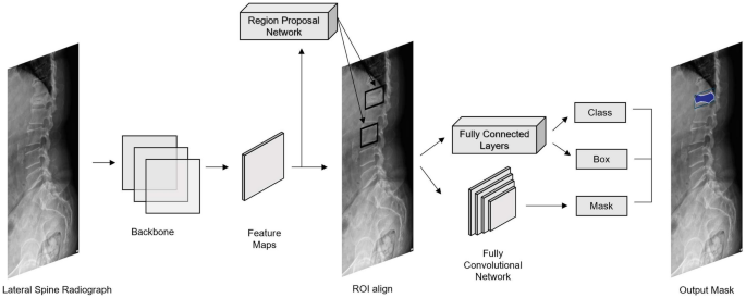
Mask R-CNN is an instance segmentation model based on the Faster R-CNN model.19Mask R-CNN20 To handle instance segmentation, we introduced a segmentation branch consisting of 4 convolutions, 1 deconvolution, and 1 convolution. In addition, ROI Align was introduced to correct the information loss of ROI pooling due to the misalignment of feature maps and ROIs (Regions of Interest), greatly improving the segmentation accuracy. The backbone of Mask R-CNN is ResNet.twenty one and Feature Pyramid Networks (FPN)twenty twoThe backbone used residual learning to accurately extract object features, and then used feature pyramid to fuse multi-scale features to build a high-quality feature map. Then, region proposal networks were used to extract ROIs from the feature map. The ROIs were then aligned and pooled by ROI Align. After the pooling layer, the model used a fully convolutional network to predict the segmentation mask. The structure of Mask R-CNN is shown in Figure 2. Mask R-CNN has several applications in instance segmentation. Mask R-CNN takes the structure of the previous RCNN model and improves it to be a faster, more accurate and effective instance segmentation model.

Mask R-CNN model architecture.
Backbone Network
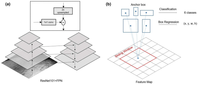
The backbone network was used to extract features from the input radiographs. To extract reliable feature maps, we implemented ResNet101 with FPN as the backbone network. In the bottom-up pathway, ResNet extracts low-level features such as object corners and edges, while deeper layers extract higher-level features such as texture and color. Then, in the top-down pathway, FPN was used to concatenate feature maps at different scales to better represent the object. The feature maps were used by RPN and ROI Align to generate candidate region proposals for detection. The structure of the backbone network is shown in Figure 3.
Local recommendation network and ROI are aligned
The RPN generates ROIs using the feature map input from the backbone network. A 3 x 3 convolutional layer is used to scan the image using a sliding window to generate bounding box anchors at different scales. Binary classification is performed to determine whether each anchor contains an object or represents the background. The structure of the RPN is shown in Figure 3. Samples were generated by bounding box regression and the intersection over union (IoU) value was calculated. If the IoU of a sample was greater than 0.7, it was defined as a positive sample, otherwise it was a negative sample. Non-maximum suppression (NMS) was applied to retain the region with the highest confidence score. The feature map from the backbone network and the ROI from the RPN were passed to ROI Align for pooling. In the next stage, ROI Align was performed to obtain a fixed-size feature vector and feature map. ROI Align rounds the position of the ROI on the feature map in a proposed way to avoid the misalignment problem identified in the ROI pooling layer. Prior to pooling, a bilinear interpolation operation was performed on the sample points within each grid cell.
Mask Prediction
The output feature vectors from the previous stage were used to calculate class probabilities for each ROI for classification, and a bounding box regressor was trained to adjust the bounding box position and size to accurately contain each object. The mask branch used a fully convolutional network (FCN) to predict a binary mask for each ROI per class.

Backbone network and region proposal network.One) The backbone network is shown. The feature maps of the ResNet are upsampled and resized with 1 x 1 convolutions and concatenated with feature maps of different scales. (b) The region proposal network generates candidate object regions, called anchor boxes, on the feature map through a sliding window. Each anchor box performs both classification and bounding box refinement.
Evaluation Metrics
True positives and false positives were defined by the value of IoU. IoU was calculated by dividing the overlap of the predicted and actual regions by their sum. If the IoU of the predicted and actual regions exceeded a certain threshold, the detector's prediction was determined to be correct and was defined as a true positive (TP). Conversely, if the IoU value was less than the threshold, it was defined as a false positive (FP). If the detector failed to predict a fracture, it was defined as a false negative (FN). Specificity was calculated using a dataset that did not contain any fractures. If the detector did not predict a fracture from a normal radiograph, it was defined as a true negative (TN), and a false positive was defined as a false positive (FP). Using the defined confusion matrix, we calculated the sensitivity, specificity, accuracy, and F1 score. Sensitivity is calculated by Equation (1), specificity by Equation (2), accuracy by Equation (3), and F1 score by Equation (4)
The cumulative value was determined by listing the detected regions in order of their confidence scores. Once the regions were listed, the cumulative value was used to calculate the precision-recall curve and the AP was calculated from the area under it. The mean precision (mAP) was calculated as the average AP score for each class and evaluated as an overall evaluation metric among each DL model. The AP score was calculated by Equation (5):
$$\begin{aligned} Sensitivity&= \frac{TP}{TP + FN} \end{aligned}$$
(1)
$$\begin{aligned} specificity&= \frac{TN}{FP + TN} \end{aligned}$$
(2)
$$\begin{aligned} Accuracy&= \frac{TP + TN}{TP + FP + TN + FN} \end{aligned}$$
(3)
$$\begin{aligned} F1 score = 2 * \frac{precision \times recall}{precision + recall} \end{aligned}$$
(Four)
$$\begin{aligned} AP&= \frac{1}{6}\sum _{confidence} precision(recall) \end{aligned}$$
(5)
Ethics approval and consent of participants
This study was conducted in accordance with the Declaration of Helsinki. This study was approved by the Institutional Review Board of Korea University Ansan Hospital and was conducted in accordance with the approved research protocol (IRB No. 2022AS0198). As this study is retrospective, informed consent was exempted from the Institutional Review Board of Korea University Ansan Hospital and the Institutional Review Board.


