

Dataset Description
A data set of 60 tissue microarrays (TMAs) was used. Each contains a single core for each case, with 20 cases representing each diagnosis (cancer, health, and goiter). These TMAs were acquired from Microarray Inc. in Rockville, USA, and consist of both male and female patients ages 17 to 80, ensuring age and gender diversity. The cancer group includes both papillary and follicular thyroid cancer cases, but the goiter group consists of a variety of benign conditions, including nodular goiter, diffuse toxic goiter, Hashimoto's thyroiditis, subactive thyroiditis, and fibrous thyroiditis. Tissue samples were initially pre-labeled by a company pathologist and then verified and confirmed by two experienced pathologists specializing in thyroid tissue.
These tissues were later used to measure the absorbance spectra of each small portion corresponding to the voxel. These measurements used a Perkinelmer Spotlight 400 Micro-ftiR spectrometer equipped with a microscope to assess absorbance intensity of thyroid tissue over an infrared spectral range of 778-1800 cm.-1. Most of the captured images were about 300 x 300 pixels in size and had slight variations in dimensions. Through spectral mapping, data were collected at two wavenumber intervals and intensity measurements of 512 per voxel were made. The system provided a spectral resolution of 4 cm.-1 Spatial resolution of 6.25μm. To ensure accuracy, hyperspectral imaging (HSI) data were acquired under tightly controlled conditions and relative humidity was maintained below 5% using dry air.
Pre-processing
A five-stage preprocessing pipeline was developed to improve the quality of the data and to remove unrelated information (Figure 1). The goal of this pipeline was to segment regions of interest (ROIs), such as cellular structures, while eliminating unnecessary components (e.g. other thyroid structures, such as colloids). First, each spectral band was normalized to the range 0-1 using MIN-MAX scaling. The resulting spectrum was multiplied by 255 to convert it to an integer to generate pixel values, allowing each spectral band to be visualized as a grayscale image.
We then selected representative spectral bands (Fig. 1 – STEP 1) that distinguished tissue internal structures, particularly other elements such as colloids. I chose 1624 cm-1 The band is within the spectral region known as amide I (approximately 1590-1690 cm).-1), is associated with protein c=o stretch vibrations. This absorption is strongly expressed in cellular structure due to the high protein content of thyroid follicular cells. In contrast, colloids are composed primarily of glycoproteins, with fewer peptide bonds and weaker absorption in this region.twenty one. Converting each spectral band into a grayscale image gives 1624 cm-1 The band provided the greatest visual contrast between the cells (high absorption) and the colloid (low absorption).
I then converted the grayscale image at 1624 cm-1 Fast Fourier Transform (FFT) is used to enter the frequency domain (Figure 1 – STEP 2). This transformation allows for image analysis based on spatial frequency components. After that, a high-pass filter was applied to emphasize the high-frequency components and suppress the low-frequency components (Figures 1 to 3). This step was important for increasing the visibility of fine tissue details and cell boundaries.
Following high-pass filtering, a threshold was applied with a value of 127 to separate the background and regions of interest (Fig. 1 – Step 4). This process primarily emphasized the cell nuclei and was able to focus on key features within the tissue. However, to capture a more comprehensive spectrum of the entire cell structure, we employed a 3×3 extension kernel in one iteration to expand the detected regions (Fig. 1 – STEP 5). This expansion has improved cell structure visibility and has provided a more accurate representation of cell structure within tissues.
Because these regions were considered more representative of cellular structures within tissues, we chose voxels that correspond only to the white areas of the segmentation mask. This focused approach ensured that the analysis was based on the most relevant data. Selected voxels were used for pattern recognition using 1D-CNN. In total, we obtained 104,107 voxels for this analysis, providing a robust dataset that enhances the accuracy and effectiveness of pattern recognition efforts.
Finally, we augmented the dataset by adding Gaussian noise to the existing samples. This addition of Gaussian noise is beneficial in increasing the robustness of the model as it helps to simulate actual variation and improve the ability of the model to generalize to invisible data. By incorporating this noise, we effectively doubled the training dataset, increasing its variability, and contributed to the generalization of the overall model. It is important to note that we apply extensions to training samples only, ensuring that the test dataset is not modified and only retains the original preprocessing.
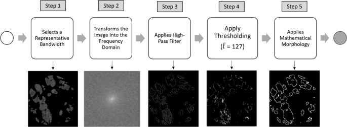
The proposed pipeline for ROI segmentation of HSI.
Classification methodology
In our comparative study, we analyze three distinct deep learning architectures applied to classification of thyroid tissue using hyperspectral imaging: FCNN (Figure 2A) and LSTM-RNN (Figure 2B) are previously developed and tested and newly developed architectures, 1D-CNN (Figure 2C). These architectures were developed through empirical experiments. For FCNNs, grid searches were performed to optimize key hyperparameters such as activation function, loss function, optimizer, and number of neurons per layer. These optimized configurations provided a strong baseline and used it as a reference point to guide tweaking of LSTM-RNN and the newly proposed 1D-CNN architecture.
FCNN is designed with eight layers, one input layer, six hidden dense layers, and one output layer. The input layer contains 100 neurons corresponding to 100 frequencies selected using the SelectKBEST algorithm. This method was the only method that used dimension reduction. LSTM and 1D-CNN were not used due to their nature to process long sequences of data. Each of the six hidden layers of FCNN have 86 neurons, all employing a modified linear unit (Relu) activation function. The output layer consists of three neurons representing one of the classes of research with softmax activation functions.
The LSTM-RNN model consists of two layers, including 256 LSTM units and a second 128 units. Each LSTM layer is followed by a dropout layer deactivating 20% of the neurons. This model handles the entire range of hyperspectral data, consisting of 512 intensity values per frequency. The output layer contains three neurons corresponding to three classification labels.
Finally, the newly proposed 1D-CNN architecture is set up as follows: It consists of a total of six layers. The input layer receives an intensity value of 512, followed by two convolutional layers extracting 16 and 32 filters, both using three filter sizes. These values are empirically defined based on experimental results and are intended to balance architectural complexity with model performance. After each convolution operation, a 1D spatial dropout is applied, randomly disabling 40% of the neurons in that layer, and disabling the 1D maximum pooling operation of two sizes. The purpose of this sequence is to reduce the dimensions of the data, thereby reducing the risk of overfitting, while maintaining the essential properties.
A combination of these operations gives a total of 4032 1D functional maps from the convolutional layer. These features are then flattened and trained with a multilayer perceptron (MLP). The MLP consists of three dense layers. The first layer has 4032 neurons, the second has 100 neurons, and the three neurons have 3 neurons. The hidden layers use Relu Activation Function, while the output layers perform classification by assigning a probability to each input using the SoftMax function, indicating the possibility of belonging to one of three predefined classes.
Additional parameters include Adam Optimizers selected for efficiency in adapting learning rates, making them particularly suitable for large datasets with many parameters. L2 regularization is implemented to minimize the risk of overfitting by adding a penalty period that promotes lower body weight values within the network. The batch size is set to automatic, allowing the system to determine the most efficient value and optimize the use of computational resources. Finally, the network trains over 5000 epochs to ensure robust learning and model performance.

(a)fcnn, (b)lstm-rnn and (c) 1D-CNN Architecture Scheme.


