Case study
Taiwan’s water quality monitoring system was selected as the case study for this research due to its comprehensiveness and relevance to water resource management in the region. The system is managed by Taiwan’s Environmental Protection Administration and covers rivers, reservoirs, and lakes nationwide, focusing on assessing, reporting, and improving water quality66.
Taiwan is an island with an area of approximately 36,000 \(km^2\), characterized by diverse geography, including mountains, plains, and coastal areas. The island’s hydrographic network comprises 151 major rivers and numerous reservoirs and lakes of significant environmental and economic importance. Water quality monitoring focuses on water bodies that provide drinking water, are used for irrigation, or have ecological significance.
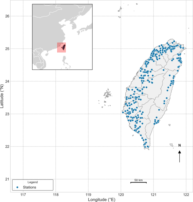
Water quality data is regularly collected at over 500 monitoring stations strategically distributed across the territory, covering physico-chemical and biological parameters such as dissolved oxygen, Biochemical Oxygen Demand (BOD), nitrogen, phosphorus, suspended solids, and fecal coliforms, among others. The locations of the monitoring stations used are described in Figure 1, where the stations are situated in the country’s reservoirs, specifically those with higher sampling frequencies, totaling 306 monitoring stations. This dataset, which has been continuously and publicly available since 1987, provides a robust foundation for developing and validating ML models for water quality assessment and prediction.

Map of sampling station locations. Map generated by the authors using Python source code with openly available data66.
The monitoring network was implemented to address the growing need to protect the island’s water resources from the impacts of human activities, including intensive agriculture, urbanization, and industrialization. In recent years, significant improvements in water quality have been observed across several river basins, driven by the implementation of strict pollution control policies and investments in sanitation infrastructure.
Taiwan’s system also stands out for its use of technology, including real-time sensors and early warning systems, which enable the rapid identification of changes in water quality and effective responses to pollution incidents. This study aims to leverage these historical and real-time data to enhance the application of ML-based models in water quality monitoring and management in Taiwan.
Data description
The original dataset66 consists of 18 variables, as shown in Table 2. For this study, the relevant columns are: siteid” and sampledate”, which identify each measurement instance; and itemengabbreviation” and itemvalue”, which contain the recorded data. The values in the “itemengname” column denote the different measurement types collected, as listed in Table 3.
The main variable of interest is the River Pollution Index (RPI), which serves as a proxy for the Water Quality Index (WQI) in this study. The RPI is a composite measure that integrates various physicochemical parameters into a single value, enabling a comprehensive assessment of water quality and pollution levels. In the analyzed dataset, RPI values range from 1.0 to 7.3, covering conditions from clean to heavily polluted waters.
The predictor variables selected for water quality assessment are electrical conductivity (EC), suspended solids (SS), water temperature (WT), and pH. The choice of these variables is grounded in established literature31,32. EC reflects the concentration of dissolved ions and serves as an indicator of contamination from domestic, industrial, and agricultural sources. High EC values typically correspond to lower water quality.
SS refers to particulate matter suspended in the water column, which contributes to turbidity, limits light penetration, and can transport harmful substances. Elevated SS levels may result from erosion, runoff, or waste discharge.
WT plays a vital role in regulating chemical and biological processes in aquatic systems. It affects oxygen solubility, the metabolism of aquatic organisms, and the balance of nutrients and toxins. Significant temperature variations may signal human influence and impact overall water quality.
A key indicator of water quality, pH reflects the acidity or alkalinity of water and influences the chemical balance in aquatic ecosystems. Changes in neutral pH levels can affect nutrient availability, increase the risk of toxic substances, and harm aquatic organisms, often signaling human-induced stressors such as industrial discharges or eutrophication.
Table 4 summarizes the descriptive statistics of the selected variables, showing variation in pollution levels and environmental conditions across the dataset.
Data preprocessing
The preprocessing phase begins with the selection of key variables for analysis, namely Electrical Conductivity (EC), River Pollution Indicator (RPI), Suspended Solids (SS), Water Temperature (WT), and pH. These variables were chosen due to their ease of collection and cost-effectiveness, eliminating the need for laboratory sample processing. The dataset’s Itemvalue attribute, initially stored as text, is converted into a numeric type. During this conversion, any values that could not be parsed as valid numbers were marked as missing by assigning them the null token NaN. After this step, we identified and removed all samples (rows) with one or more missing values in the selected variables (EC, SS, WT, pH, or RPI). This ensured that only complete and reliable records were used for model training and evaluation. The dataset is then partitioned into training and testing sets. The independent variables (EC, SS, WT, pH) serve as predictors of the dependent variable RPI.
To split the dataset into training and testing sets, a random division strategy was adopted for each execution, with 75% of the samples allocated for model training and 25% for testing. Additionally, the model was run 100 times, each execution using a distinct random seed in order to evaluate how the model performs under different environmental conditions. Since the dataset comprises measurements collected from multiple monitoring stations, with varying sampling schedules and geographic locations, a chronological split would not ensure temporal continuity or consistency across all stations. This random approach is more appropriate for the current dataset, as it better preserves the distribution and diversity of the samples, thereby avoiding biases associated with specific periods or geographic regions. Furthermore, since the objective is to model general relationships between water quality parameters and the River Pollution Index (RPI), rather than predicting future values in a temporal sequence, chronological order is not essential. Random splitting helps ensure that the training and testing sets are more representative, supporting the development of a more consistent and generalizable model across different spatial and temporal contexts.
Automated machine learning
ML models can be categorized into two main groups: supervised learning and unsupervised learning. In supervised learning, the dataset consists of input attributes associated with corresponding output values, and the objective is to identify a function that maps the input data to these outputs. In unsupervised learning, the goal is to organize the data based on inherent similarities, as there are no predefined labels to guide the organization process. Within supervised learning, when the output values are categorical, classification models are employed. When the outputs are numerical, regression models are used. Beyond these fundamental methods, it is common practice to combine predictions from multiple models to improve overall performance. This approach is referred to as ensemble, which includes techniques such as bagging67, boosting68, and stacking69.
When applying ML models for prediction tasks, several challenges arise, including data preprocessing, model or ensemble selection, hyperparameter tuning, and feature engineering. To address these challenges, AutoML methods have been developed to automate these steps, creating an end-to-end pipeline for training ML models.
In this study, the open-source platform AutoGluon52 was used to select ensembles of models from the scikit-learn library70 to predict the water quality index.
AutoGluon
AutoGluon52 is an open-source platform developed by Amazon to facilitate the application of AutoML for regression and classification problems. The platform is designed to simplify the construction of model ensembles, without requiring manual hyperparameter tuning or complex pipeline configuration. Its primary approach is to combine multiple models into ensembles and stack them in multiple layers to enhance prediction performance, a method known as multilayer ensemble, as reported in Figure 2: In the first layer, a set of base models is trained using the input data. The predictions from the first-layer models are then used as additional features to train the models in the next layer.

Multilayer ensemble used in AutoGluon71.
For example, if the first-layer models receive ten input features, the next-layer models will receive the same ten features plus the outputs of the models trained in the previous layer. This allows higher-layer models to revisit the original data during training and learn residual patterns and errors from the previous layers. To maintain simplicity, AutoGluon reuses the same model types (including their hyperparameters) from the base layer in subsequent layers.
Finally, the last layer aggregates the predictions of the previous layer’s models using weighted averaging, where each model’s output is weighted based on its contribution to the overall ensemble performance. In addition to the multilayer ensemble approach, AutoGluon proposes using repeated k-fold bagging (also known as cross-validation committees) to further reduce the variance of the final model72. If sufficient training time is available, the k-fold bagging process is repeated n times with different random partitions of the dataset. The goal is to create diverse and robust base models while improving the performance of the final ensemble.
AutoGluon also automates critical preprocessing steps to enhance model stability52. Indeed, it automatically handles missing values through median/mode imputation for numerical features and learned imputation strategies for categorical features. The platform performs automatic feature scaling (standardization and normalization) to ensure numerical features are on comparable scales, which is essential for distance-based algorithms, such as k-NN. For categorical features, AutoGluon applies optimized encoding strategies including one-hot encoding, ordinal encoding, and target-based encoding. Lastly, the system also automatically generates feature interactions and polynomial features to capture nonlinear relationships. Such preprocessing operations occur transparently within the training pipeline without requiring manual configuration.
The platform supports a variety of model types, including k-Nearest Neighbors (k-NN), linear regression, ANNs, boosting tree methods (e.g., GBM-based methods), bagging methods (e.g., RF), and extremely randomized trees.
k-nearest neighbors
The k-NN73 algorithm exploits the intuition that observations with similar characteristics will lie close together in the feature space. Given a new instance, the method first computes distances – typically Euclidean, though alternatives (e.g., Manhattan or Minkowski) can be used. Owing to its straightforward logic, k-NN is straightforward. It makes observations with the smallest distances. For classification tasks, the predicted label is determined by a majority vote among these k neighbors; for regression tasks, it is given by the average target value of these k neighbors. The following flowchart (Figure 3) visually summarizes the steps involved in the k-NN algorithm, from computing distances to determining the predicted label or value.
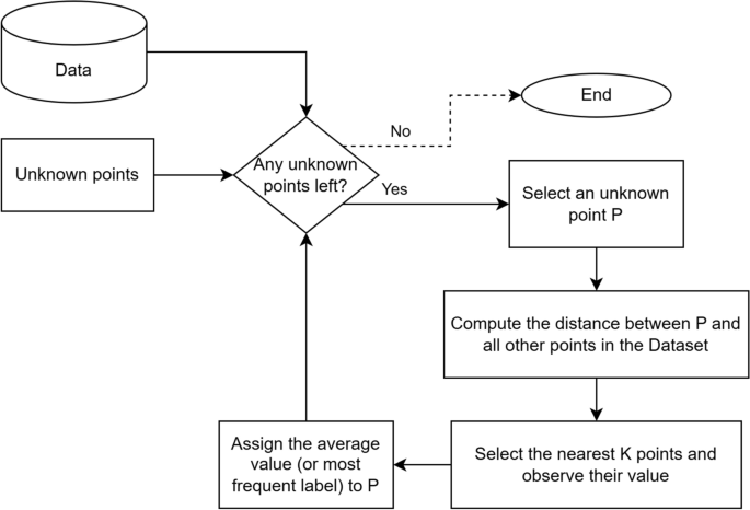
Flowchart of a k-NN model.
Thanks to its straightforward logic, k-NN is exceptionally simple to implement and interpret. It often delivers strong performance on small to medium datasets and naturally extends to multi-class problems without modification. As a non-parametric method, it makes no explicit assumptions about the underlying data distribution, allowing it to adapt flexibly to complex decision boundaries. Moreover, since k-NN defers all “learning” to prediction time, it requires no costly training phase – models are built implicitly by storing the entire training set and indexing it for fast neighbor retrieval.
However, the above-described strengths also entail key limitations. Prediction can be computationally expensive when the training set is large, as distance calculations must be performed against every stored example. Memory requirements likewise grow linearly with dataset size, potentially leading to scalability challenges. Performance is highly sensitive to the choice of distance metric and the hyperparameter k: selecting a very small k can yield noisy, high-variance predictions. In contrast, a very large k may oversmooth the decision boundary and introduce bias. Careful validation is therefore essential to strike the appropriate balance between bias and variance and to select a distance measure aligned with the problem domain.
Linear regression
The Linear Regression model74 seeks to capture a direct, proportional relationship between a continuous target variable Y and one or more input features \(X_n\) (Equation 1). In its simplest formulation, model parameters are chosen to minimize the sum of squared differences between the observed outcomes and the values predicted by the linear predictor (Equation 2). In small-to medium-scale problems, this can be achieved by solving the ordinary least squares criterion in closed form; when datasets grow large or feature dimensionality is high, one often resorts to iterative approaches such as Gradient Descent to obtain the optimal coefficients. In equations 1 and 2, \(y_i\) and \(x_{in}\) denote the i-th sample of the \(X_n\) and Y arrays.
$$\begin{aligned} y_i = \beta _0 + \beta _1 x_{i1} + \cdots + \beta _{n} x_{in} \end{aligned}$$
(1)
$$\begin{aligned} \varepsilon = \min \sum _{i=1}^k (y_i – \beta _0 – \beta _1 x_{i1} – \cdots – \beta _n x_{in})^2 \end{aligned}$$
(2)
The validity of Linear Regression rests on several core assumptions. First, the effect of each feature on the target must be additive and proportional, so that a change in a predictor produces a constant change in the response. Second, the residual errors (the differences between actual and predicted values) should be mutually independent, have constant variance across all levels of the predictors (homoscedasticity), and ideally follow a normal distribution to support reliable hypothesis testing and interval estimation. Third, the explanatory variables themselves should not exhibit excessive collinearity, since highly correlated inputs can inflate the variance of the estimated coefficients and undermine interpretability.
Despite its conceptual simplicity and ease of interpretation, Linear Regression is notably sensitive to outliers, which can disproportionately skew the fitted relationship. It also struggles in settings where the true mapping between inputs and outputs is nonlinear, or when the error distribution departs substantially from normality. In practice, these limitations are often addressed through robust regression methods, feature transformations (such as polynomial or interaction terms), or regularization techniques (Ridge or Lasso) that penalize large coefficients and help stabilize estimates in the presence of multicollinearity. An illustrative example of Linear Regression is presented in Figure 4.

Example of a linear regression model.
Artificial neural networks
ANNs are ML models inspired by the structure and functioning of the human brain75. In particular, their architecture consists of layers of artificial neurons interconnected to process information and learn patterns from data76: for instance, due to their ability to approximate complex functions, ANNs are widely used for tasks such as image processing77,78, natural language processing79,80, and time series forecasting53,81.
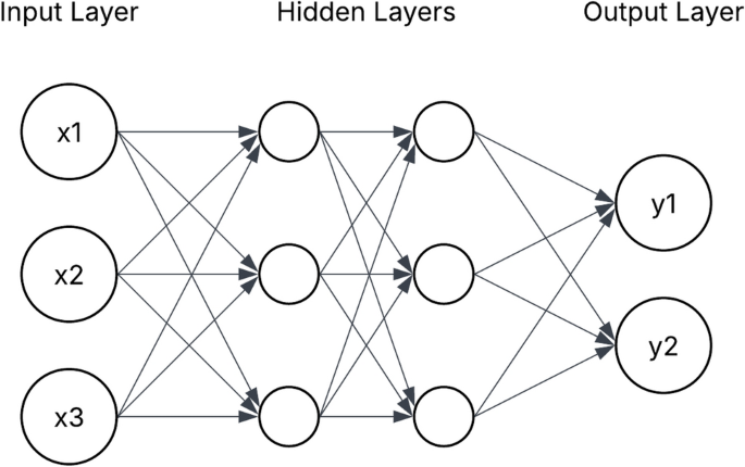
A comprehensive overview of neural networks, from their basic structure to the challenges in training and implementation, can be found in Hastie et al.82. The architecture of ANNs comprises three main types of layers: the input layer, hidden layers, and the output layer (Figure 5). The input layer receives the data, which is then processed by the hidden layers through combinations of neuron weights and activation functions. The output layer produces the final predictions or classifications.
Among activation functions, the most commonly used are sigmoid, hyperbolic tangent (tanh), and the Rectified Linear Unit (ReLU). The sigmoid function smooths the output to values between 0 and 1. However, it has limitations: (i) for extreme input values (very large or very small), the output approaches 0 or 1, causing the gradient to vanish and leading to the vanishing gradient problem; (ii) since it is not centered at 0, gradients may be biased toward positive values, which can hinder convergence during training. Despite these limitations, the sigmoid function remains widely used in tasks such as logistic regression and binary classification output layers.
The hyperbolic tangent (tanh) function is an extension of the sigmoid function, normalizing values between \(-1\) and 1. Unlike the sigmoid, tanh is centered around 0, allowing the activation outputs to have a mean close to 0. This property facilitates convergence during training, as gradients are not biased toward a specific direction. However, tanh still suffers from the vanishing gradient problem at extreme input values and is computationally more expensive.
The ReLU function is currently the most popular activation function in deep neural networks due to its computational simplicity and training efficiency. It introduces non-linearity into deep learning models, enabling neural networks to capture complex relationships in the data. Key characteristics of ReLU include: (i) it is defined in the interval \([0, +\infty ]\), where negative values are ignored and mapped to 0; (ii) it returns the input value if it is positive. This behavior helps avoid the vanishing gradient problem. However, ReLU can suffer from dead neurons, where gradients tend to zero. To address this, variants such as Leaky ReLU83 and Parametric ReLU84 have been proposed.
The training process of neural networks is based on minimizing the cost function, which measures the difference between the network’s predictions and the expected values. This is achieved using the backpropagation algorithm, which adjusts the network’s weights by propagating gradients of the cost function with respect to each weight. Weight updates are performed using gradient descent, which adjusts parameters in the direction that minimizes the error.
Despite their strong generalization capabilities, neural networks are prone to overfitting, in which they excessively fit the training data, thereby impairing their ability to generalize. To mitigate this, regularization techniques, random neuron dropout (also known as dropout), and activation normalization are commonly employed. Additionally, the choice of hyperparameters, such as the number of layers, the number of neurons, and the learning rate, can significantly influence the network’s performance.
Boosting
Boosting techniques aim to create models by sequentially combining multiple weak models. The concept was initially proposed by Schapire68, who explored the potential of weak learners (models whose hypotheses are slightly better than random predictions) and how to combine them to improve accuracy (Figure 6).
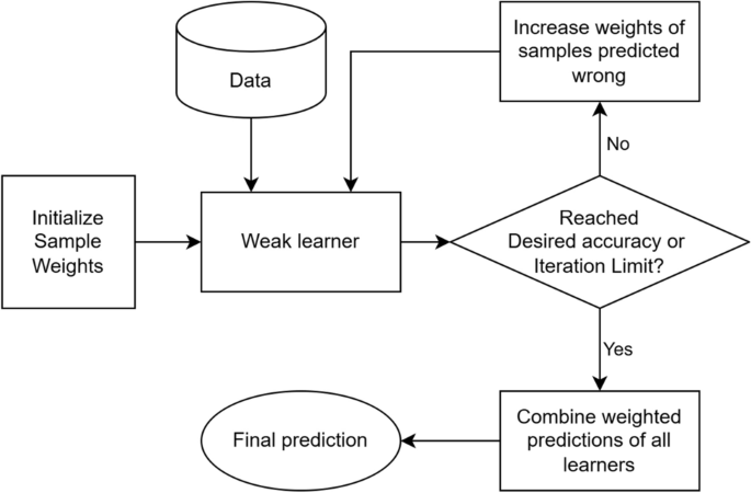
Example of a boosting model.
Subsequently, more well-known methods were developed, such as AdaBoost85, which assigns weights to training samples and adjusts them based on the model’s errors from the previous iteration. The more challenging a sample is to predict, the higher its weight in the next model.
Similarly, the Gradient Boosting method86 seeks to identify complex samples for the models by calculating residual errors at each iteration. The residual is the difference between the observed value and the current model’s prediction for each sample. In each iteration, a new tree model is trained to minimize the residual error from the previous iteration.
Given the computational cost of Gradient Boosting, where training time increases linearly with the number of trees in the model, two optimized variations were proposed: XGBoost87 and LightGBM88: XGBoost prioritizes training speed through parallelized tree construction and efficient memory usage. Additionally, to reduce overfitting, XGBoost introduces L1/L2 regularization, which penalizes the cost function to discourage overly complex trees. Similarly, LightGBM (LGBM) aims to improve scalability and performance, particularly for large datasets. Its training process supports parallelism and GPU processing, and the tree construction method uses leaf-wise growth instead of the conventional level-wise growth used in GBM. This results in deeper and more efficient trees during training.
Another method based on Gradient Boosting is Categorical Boosting (CatBoost), introduced in Prokhorenkova et al.89. Its proposal addresses the challenges of handling categorical variables and target leakage (prediction shift) in existing boosting algorithms. Additionally, CatBoost automatically handles categorical variables during training by utilizing target statistics. It introduces a temporal concept for training samples, inspired by online learning processes, creating a sequential data behavior. For each instance, the cumulative average of previous observations is calculated and used as the numerical value for each categorical variable.
Bagging-bootstrap aggregating models
As described in Breiman67, Bagging models (Bootstrap Aggregating) consist of an ensemble of decision tree models trained independently on random subsets of the original training data, sampled with replacement. Each base learner sees a slightly different view of the training set, which decorrelates their errors and leads to a more robust aggregate predictor. The goal is to reduce variance and, consequently, the tendency toward overfitting by aggregating the predictions of all independent models, typically by averaging for regression or by majority voting for classification tasks. Figure 7 illustrates the general workflow of a bagging approach. In particular, a prominent example of this class of models is the Random Forest90, where, in addition to drawing random subsets of the data (bagging), one also selects random subsets of features at each split. This additional layer of randomness further reduces correlation among individual trees, allowing each small tree to capture distinct structures and interactions within the data. The combination of bagged data samples and feature subsetting endows Random Forests with high predictive accuracy, resilience to noisy inputs, and an inherent measure of variable importance.
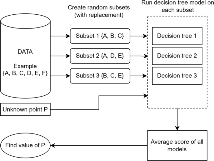
Example of a bootstrap aggregating model.
Extremely randomized trees
The method known as ExtraTrees91, short for Extremely Randomized Trees, was proposed to further increase randomness in tree construction, with the primary aim of mitigating overfitting effects. Unlike Random Forest, ExtraTrees builds each tree on the entire dataset rather than on bootstrap-sampled subsets. Moreover, during tree induction, the node-splitting process is not based on an exhaustive search for the optimal threshold: instead, for each candidate feature, split thresholds are drawn uniformly at random from within the feature’s observed range, and the best among these random thresholds (according to a chosen impurity measure) is selected. Figure 8 illustrates the general workflow of an ExtraTrees model. This pure randomization at both the data-use and split-selection stages dramatically lowers inter-tree correlation, thereby reducing variance without relying on Bagging. As a result, ExtraTrees achieves high predictive accuracy and robustness to noise, while often offering substantially faster training times.

Example of an extremely randomized trees model.
Computational experiments
The computational experiments evaluated the performance of predictive models using the AutoGluon library on a water-quality dataset in Taiwan. To ensure the reliability of the results, multiple runs of the experiment were conducted, each with a distinct random seed, thereby introducing variability and enabling a more comprehensive analysis across different scenarios.
For model training, the TabularPredictor class from the AutoGluon library was used. The problem was configured as a regression task, with the evaluation metric set to \(\hbox {R}^2\). Each model was trained for up to 20 (twenty) minutes, allowing AutoGluon to automatically explore different algorithms and hyperparameters. To optimize computational resource usage, up to 8 CPU cores were allocated for parallel training, thereby improving efficiency.
After each run, the trained models were evaluated using the following metrics: correlation coefficient (R), coefficient of determination (\(\hbox {R}^2\)), root mean squared error (RMSE), mean absolute error (MAE), and mean absolute percentage error (MAPE). In particular, Table 5 presents the equations of the employed evaluation metrics, where \(\widehat{y_i}\) denotes the predicted output, \(y_i\) represents the target, \({\overline{y}}\) is the target average, N is the total number of samples, and \(var(\cdot )\) is the variance and \(cov(\cdot , \cdot )\) is the covariance.
The employed metrics were selected to provide a comprehensive view of the models’ predictive performance, enabling a detailed analysis of prediction accuracy. Additionally, the importance of predictor variables was calculated for each model, and the results were normalized to facilitate the interpretation of the most influential factors in the predictive process. In order to ensure traceability and integrity of the results, all information was stored in JSON files. Each file contains data such as the random seed used, the trained model, performance metrics, model hyperparameters, variable importance, and the actual and predicted values for the test data. The results of each run were organized into directories, one per model, and the best-performing model was highlighted and stored in a separate directory, simplifying the identification of the top model for future analysis.
All simulations in this study were performed on a laptop equipped with an Intel Core i7-7700 K processor (4.2 GHz) and 16 GB of DDR3-2400 MHz RAM. The code executed on this hardware configuration was developed in Python (version 3.12). AutoGluon52 was used to construct and train predictive models, and the scikit-learn library70 (version 1.3) was employed for evaluation metrics.