
In this research work, a novel ArSL model is introduced, with the assistance acquired from the AI based approaches and hybrid meta-heuristic optimization model. The overall architecture of the proposed model is shown in Fig. 1.

Overall architecture of proposed approach.
Image acquisition
The proposed approach for detecting ASL includes detailed image acquisition process which is mainly based on two datasets.
Arabic Sign Language ArSL dataset
The dataset 1 (https://www.kaggle.com/datasets/sabribelmadoui/arabic-sign-language-augmented-dataset) for the image acquisition is well-prepared for developing a reliable Arabic sign language recognition system. The Arabic sign language was made up of 290 images to the test set, 13,926 images to the training set, 870 images for the validation set making a total of 15,086 images in total and every image has a dimension of 416 × 416 pixels. These images were captured in different settings with different backgrounds and different angles of hand holding the cell phone camera.
RGB Arabic Alphabets Sign Language Dataset
Dataset 2 (https://www.kaggle.com/datasets/muhammadalbrham/rgb-arabic-alphabets-sign-language-dataset) appears to be a valuable resource for image acquisition and model training. RGB Arabic Alphabet Sign Language (AASL) database includes 7857 raw and fully labelled RGB images for Arabic sign language alphabets, that, to the knowledge, was the first public RGB database. The database has been expected to be useful to anyone who wants to build realistic Arabic sign language classification models. The dataset is intended to assist anyone who are interested in creating classification models for Arabic sign language in real-world scenarios. More than 200 individuals’ AASL was gathered under various conditions, including background, illumination, image orientation, size, and resolution. To guarantee a high-quality dataset, the gathered photos were supervised, verified, and filtered by subject-matter experts.
KArSL database
Dataset 3, can be downloaded from: https://www.kaggle.com/datasets/yousefdotpy/karsl-502. KArSL is one of the largest video databases for width-Arabic sign language. The database is built around 502 isolated sign words collected with the Microsoft Kinect V2. Each sign of the database is performed by three professional signers. Each signer repeated each sign 50 times, resulting in a total of 75,300 samples of the whole database (502 × 3 × 50).
Pre-processing
Image resizing
The collected RGB images has been resized to a standard size of 224 × 224 pixels for all the images used in the dataset. This resizing is important in order to achieve uniformity of the input size which is important for the machine learning models to process. Figure 2 represents the resized images for database 1 and database 2.

Resized images and L*a*b converted images for the samples of database 1 and database 2.
L*a*b* color space conversion
After resizing the images go through L*a*b* Color Space Conversion, which are the very important step in image processing as well as computer vision. It consists of three main components: L* which is the lightness, a* which is the redness greenness and the b* which is the blueness yellowness. In this 3D color space L* is between 0 and 100 which means black and white respectively while a* and b* are between − 128 and + 128 and represent blue-yellow and green–red respectively. L*a*b color space analysis for dataset 1 and dataset 2 are presented in Fig. 3.

L*a*b outcomes for the resized sample images.
RGB is converted directly into L*a*b* by utilizing Eq. (1)
$$\left[P\, M \,N \right]=\left[Q\right]\left[R \,G \,B \right]$$
(1)
Here Q is obtained as per Eq. (2),
$$\left[Q\right]=\left[{H}_{r}{P}_{r} {H}_{g}{P}_{g} {H}_{b}{P}_{b} {H}_{r}{M}_{r} {H}_{g}{M}_{g} {H}_{b}{M}_{b} {H}_{r}{N}_{r} {H}_{g}{N}_{g} {H}_{b}{N}_{b}\right]$$
(2)
In the above matrix, \({P}_{k}={p}_{k}/{m}_{k}\), \({M}_{k}=1\), \({N}_{k}=\left(1-{p}_{k}-{m}_{k}\right)/{m}_{k}\left(k\in \left\{r,g,b\right\}\right)\) and [H] is obtained as per Eq. (3):
$$\left[{H}_{r} {H}_{g} {H}_{b} \right]={\left[{P}_{r} {P}_{g} {P}_{b} {M}_{r} {M}_{g} {M}_{b} {N}_{r} {N}_{g} {N}_{b} \right]}^{-1}\left[{P}_{V} {M}_{V} {N}_{V}\right]$$
(3)
After the values of \(P\), \(M,\) and \(N\) are acquired, they are employed with the goal to find the values of \({L}^{*}\), \({a}^{*}\) and \({b}^{*}\). Equation (4) provides a set of formulas to obtain \({L}^{*}{a}^{*}{b}^{*}\).
$${L}^{*}=116 f\left(\frac{M}{{M}_{c}}\right)-16$$
$${a}^{*}=500\left(f\left(\frac{P}{{P}_{c}}\right)-f\left(\frac{M}{{M}_{c}}\right)\right)$$
$${b}^{*}=200\left(f\left(\frac{M}{{M}_{c}}\right)-f\left(\frac{N}{{N}_{c}}\right)\right)$$
(4)
Here, \({P}_{c}, {M}_{c},\) and \({N}_{c}\) represents the coordinates of the white reference illuminant. The function of \(f\) is defined as per Eq. (5).
$$f(u) = \{ \sqrt[3]{u} \quad if\quad u > \delta^{3} \left( {\delta = \frac{6}{29}} \right) \frac{u}{{3\delta^{2} }} + \frac{4}{29}\quad otherwise$$
(5)
Image augmentation
Following the capturing of L*a*b color space images, the images were subjected to image augmentation to increase the dataset variability and resilience. Some technologies utilized with this procedure involve rotation, flipping, and scaling among others. Rotation is performed at certain degrees like 45, 90, and 180 degrees which results to several images of the same object with different orientations to make the model rotationally invariant. The flipping is done both in the horizontal (left and right) and vertical (top and bottom) axis making it possible for the model to recognize the objects in any orientation. The scaling which is the process of enlarging or reducing the size of the images is important in helping the model learn different objects in different sizes and distances. Augmented images of dataset 1 and dataset 2 is graphically depicted by Fig. 4. The augmented image is the pre-processed image, from where the ROI regions are identified in the segmentation stage.

Augmented images of database 1 and database 2.
G-TverskyUNet3+: proposed architecture
The 3D U-Net provides the basis of G-TverskyUNet3+, while the trained new GNeXt conserve computing power, an attention gates module works as a noise filter, and the new skip connection architecture with U-Net 3+ functions as a low-level feature extractor. In general, these served as the foundation for a new attention 3D U-Net with numerous skip connections that is utilized to partition images used for Arabic sign language. The architecture of the model is shown in Fig. 5.

Block diagram of the proposed G-TverskyUNet3+ architecture for Arabic sign language image segmentation.
For image segmentation, the 3D U-Net model employs an encoder-decoder architecture, in which convolutional layers gradually increase feature channels and decrease spatial size. In order to blend high-level features from deeper layers with fine-grained information from early layers, skip connections are used. This architecture maintains spatial details throughout the upsampling process, guaranteeing precise segmentation. It works very well with 3D input graphics, including gesture data from sign language. For high-quality output, the network’s topology helps to preserve both coarse and fine features.
New GNeXt
A novel backbone called GNeXt combines Ghost Convolution and ConvNeXt to effectively extract features while lowering computational overhead. ConvNeXt optimizes for accuracy and scalability by building on ResNet with improvements from Transformer models. Ghost Convolution improves processing performance by using inexpensive convolutions to generate ghost features, which lowers the model’s parameters and effort. The GNeXt backbone maintains low processing costs while handling 3D data well. The lightweight design of the model’s framework enhances accuracy and model convergence.
A three-dimensional U-Net model constitutes the basis for this framework. This includes the primary encoder and decoder elements. The usage of the new GNeXt backbone with encoder, together with the numerous skip connections along with attention modules, are the primary distinctions between the suggested model and the original 3D U-Net. Figure 6 depicts the full building.

Block diagram architecture of proposed model.
Images in 3D Arabic sign language up to 240 × 240 × 155 voxels can be supported by the model. On the left, the encoder block executes convolutional activities, ReLU activations, and batch normalizations. Up to the final encoder block F, the input image’s size progressively reduces and its channel count rises over the course of five steps. Using transposed convolution, the convolution block in the final encoder stage receives the input, evaluated it as in the previous blocks, and then passes it towards decoder blocks for upsampling. The encoder’s upper blocks extract low-level sematic information by an input image, while the lower blocks extract high-level features. The decoder then carries out the reverse action, i.e., reconstructs the image’s original size using the up-sampling technique. In this procedure, skip connections assist backpropagate the outcomes to compute the loss while giving the network access to high-level semantic image information. In order to maximize the flow for features with the encoder and decoder blocks, skip connections were added in this model. In order to conserve a substantial number of computational resources and increase accuracy, the attention gate modules filter out a noisy information and only pass essential features.
GNeXt
ConvNeXt Backbone and Group Convolutions are combined to create the recently developed GNeXt. Using the ImageNet dataset, one of the most advanced backbone models, ConvNeXt, obtained a top-1 accuracy of 87–88%. Convolutional networks make up the entirety of the model, which retains the simplicity and efficiency for a standard CNN while outperforming Transformer by terms of scalability and accuracy. ConvNeXt builds upon the ResNet network’s basic architecture to gradually enhance the model by using Swin Transformer’s design. Additionally, a 3D version for novel GNeXt backbone is used here as an encoder block with the model for Ghost convolution, the cost-effective linear operation to build feature maps that efficiently reduces model parameters and computing workload. As shown in Fig. 7, this design is an enhanced version of MobileNetv1, with shortcut connections between bottlenecks and linear bottlenecks between layers.

The block first does a 1 × 1 × 1 convolution with ReLU6 and the batch normalization using a set of features includes width, height, and depth. Using batch normalization and ReLU6 to convolve three RGB channels, the input is processed in the second layer using a 3 × 3 × 3 depth-wise convolution, following the original architecture. However, volumetric data is employed in this instance. Consequently, since the information do not present three RGB channels, 3D depth wise voxels for 3D input image.
An additional 1 × 1 × 1 convolution is done without the activation function with block’s final layer. After that, the output has been added to earlier input. Due to the high processing overhead associated with 3D convolutions, this block aids in the model’s ability to remain small. This allows for low-cost, depth-wise convolution to extract by many features as possible by an input image at every stage. Additionally, new GNeXt with 3D pretrained weights is employed, and the transfer learning technique is applied. This approach improved the accuracy slightly while enabling the model to converge more quickly and smoothly than previous models.
Ghost convolution
Model parameters and computational workload were dramatically reduced when GhostNet developed Ghost convolution, a linear process that generates feature maps at a low cost.
The design of Ghost convolution is shown in Fig. 8, where the conventional convolution operation is split into two parts: the primary convolution as well as cheap convolution. The primary convolution severely restricts the total number of kernels used in convolution could be significantly less than which of traditional convolution, else it is practically the same as conventional convolution. Cheap convolution, on the other hand, performs group convolution using the original feature map that is produced by primary convolution, producing redundant feature maps that are referred to Ghost feature maps. Group convolution drastically lowers the complexity of the model by using less computation and operating more quickly than ordinary convolution. To create output feature maps necessary for feature extraction, the primary and Ghost feature maps has been combined. The primary and the Ghost feature maps were maintained at same size with this method. Ghost convolution used several times throughout the network to avoid the object detector producing an excessive number of parameters.

Architecture of Ghost convolution.
There are 1:1:9:1ratios of ConvNeXt blocks in each step. In addition, the first down sampling module creates the Patchify layer using a convolutional layer with a 4 × 4 kernel size. Compared to ResNet, the ConvNeXt block has an inverted bottleneck structure and a bigger 7 × 7 kernel size. The layer normalization (LN) layer and Gaussian error linear units (GELU) function as per Eq. (6), which are employed in Transformer, take the place of the widely utilized batch norm (BN) and ReLU activation function with CNN in microscopic architecture, resulting in fewer layers. Between the two 1 × 1 convolution layers in the block and the one LN layer that comes before the convolutions layer, there is only one activation layer that remains. Additionally, a separate 2 × 2 convolutional down sampling layers with a stride of 2 is employed, and to stabilize the training, an LN layer is added afterwards.
$$GELU\left(x\right)={x}^{*}\Phi \left(x\right)$$
(6)
In Eq. (6), Φ(x) represents as Gaussian distribution’s cumulative distribution function.
Multiple skip connections
The problem of disappearing gradients in deep networks is addressed by multiple skip connections, which enhance information flow between encoder and decoder layers. Fine-grained details are preserved by these connections, which enable low-level information from the encoder to be sent straight to the decoder. The model ensures accurate segmentation by capturing both coarse and fine information through the use of skip links throughout the network. Deeper networks can avoid losing important information during the upsampling process thanks to this strategy. The accuracy of the model is improved by skip connections, particularly for intricate tasks like gesture recognition. The 3D version deep method is employed, which enables modules to extract more high-level features with high accuracy; however, deeper networks use a less efficient backpropagation technique, which affects how the loss is calculated. For the Res-Net and U-Net algorithm, skip connections have been successfully offered as a solution to this issue. In order to address the disappearing problem and deteriorating accuracy with Res-Net, the skip connections skip across one or more levels along with its associated activities. Traditional neural network framework starts by summing the input and weights with an output from the preceding layer, \({X}_{0}\), and then activate the input using the activation function. Then, the procedure typically repeats twice, as per Eq. (7).
$$\begin{aligned} & Z_{1} = W_{1} X_{0} + b_{1} \to X_{1} = ReLU\left( {Z_{1} } \right) \\ & Z_{2} = W_{2} X_{1} + b_{2} \to X_{2} = ReLU\left( {Z_{2} } \right) \\ \end{aligned}$$
(7)
From the skip connections, repeat the same procedure but in one more mechanism. Then pass the \({X}_{0}\) and add it among with \({Z}_{2}\) with the second activation function, as represented by Eq. (8).
$${X}_{2}=ReLU({Z}_{2})$$
(8)
If all of the values are positive, the activation function immediately outputs the two inputs that were previously received. When the range of \({Z}_{2}\) is negative, then these only outputs \({X}_{0}\), and the output might be illustrated by Eq. (9).
In contrast, without skip connections, \({Z}_{2}\) with a 0 value, which will be deactivated. The network may perform convolution process with deeper networks without loss by avoiding some outputs with a range of 0. This is made possible by the skip connection operation. Nearly identical activities are needed in U-Net architecture. Rather than going towards subsequent encoder layers, the output of preceding encoder layers is transferred towards decoder layers. Furthermore, U-Net used a concatenation procedure in place of an addition operation. Later on, U-Net3+ and U-Net++ redesigned versions for skip connections were suggested. This study made use of U-Net3+ ‘s skip connection model to improve low-level feature extraction along with feature flow. The output is shared by top three decoder blocks and is presented as a skip connection at the first block. Share the output with the two decoder blocks at bottom starting from the second encoder block, then repeat the procedure until you reach the fourth encoder block. The decoder blocks go through the same procedure. Proceed by the bottom decoder block towards final decoder block this time. The top blocks share access to the outputs.
Figure 9 demonstrates the number of both encoder and decoder blocks provide numerous inputs into a single decoder block, D. By transmitting the pre-processed images to each convolution block in order to extract additional distinct features, those numerous skip connections help to protect the fine features that are extracted with every encoder and decoder block. Large maps of features are generated by decoder blocks and smaller, same-scale feature maps by encoder blocks are combined in each decoder block inside the network to capture both coarse-grained semantics and fine-grained features at full scales.

Output by encoder blocks A, B, C, and E and decoder block D.
Attention models
One of the primary modules in this study is the attention module. The attention gate’s main purpose is the score function. It outputs the score for each input after receiving the query and key as inputs. The final result is then processed using a value to establish the relative importance of each component. A weighted average of the components, which depend on key and query, sets up the attention method overall. After an effective application of the attention module in sequential acquisition of language assignments, the CNN sector developed the attention gate, referred to the Attention Gates. The attention mechanism concentrates on the most significant aspects of the input material by eliminating extraneous information. To assess each component of the input image’s importance, the Attention Gate assigns a score. This enables the model to ignore extraneous details and concentrate on key aspects. The attention mechanism improves feature extraction, which raises the effectiveness and performance of the model. It is especially useful for applications where some attributes are more crucial than others, such as sign language recognition.
The explainability of attention mechanisms is one of its most notable features. It is challenging to comprehend the logic behind predictions using traditional deep learning models, especially convolutional or recurrent neural networks, which are frequently referred to as “black-box” models. On the other hand, attention methods offer transparency by indicating which aspects of the input the model is considering while making decisions. Attention heatmaps, which show the areas of the input data that the model considers most significant, can be used to display this. These heatmaps, for instance, show the parts of the hand or body that the model concentrates on when identifying a gesture in ArSL identification. Because it clarifies for stakeholders why the model generated a specific forecast, this visual depiction increases confidence in the model.
Additionally, attention mechanisms make the model more reliable and make debugging easier. Attention visualization makes it simple to spot instances where the model is concentrating on unimportant aspects, like background or noise, which can lead to changes in the training data or model’s architecture. Attention mechanisms are particularly good at capturing long-range relationships between various sequence pieces, which might be difficult for traditional models to do in sequential data applications like sign language recognition. Convolutional Neural Networks (CNNs) and attention are combined in this study to improve the model’s performance by enabling it to prioritize significant gesture elements, increasing classification accuracy while preserving computational economy34.
Integrating CNNs with attention processes enhances explainability and model performance in the context of ArSL recognition. By assisting the network in concentrating on the most important components of a gesture, the attention mechanism improves recognition accuracy. Additionally, the model’s behavior may be better understood and interpreted thanks to its transparency, which is particularly helpful in applications involving assistive devices for the hard of hearing. In addition to producing a more successful recognition system, the combination of CNNs and attention enhances the model’s dependability and credibility, which eventually increases its applicability in real-world situations.
Unet group convolution block
Group Convolution divides the input feature map into smaller groups and applies convolution to each group independently, lowering the computing cost. This method speeds up the model and uses less memory by reducing the number of operations needed for processing. Large inputs can be handled effectively using it, particularly in settings with limited resources. Group convolution preserves the quality of feature extraction while allowing for faster processing. Lightweight models frequently employ this method to increase efficiency without compromising performance. Group convolution was implemented in AlexNet to solve the problem of limited video memory. It is currently utilized in multiple lightweight modules to reduce the number of mechanisms and parameters, as demonstrated by Fig. 10.

According to the number of channels, this approach divides the input feature map evenly into numerous groups. Then, it performs a standard convolution on every group, assuming which an input feature map \(X\in {R}^{C\times H\times W},C\) indicates the number of channels for input feature map and \(H\) and \(W\) indicate the height and width of input feature map, respectively. Similarly, the input feature map \(Y\in {R}^{{C}^{\prime}\times {H}^{\prime}\times {W}^{\prime}}, {C}^{\prime}\) indicates the number of channels for output feature map and \({H}^{\prime}\) and \({W}^{\prime}\) indicate the height and width of output feature map, respectively. The computation of conventional convolution has been evaluated by Eq. (10):
$$N={H}^{\prime}\times {W}^{\prime}\times C\times {C}^{\prime}\times k\times k$$
(10)
where \(k\) indicates the height and width of convolution kernel.
The evaluation of group convolution is represented as per Eq. (11):
$${N}^{\prime}=g\times {H}^{\prime}\times {W}^{\prime}\times \frac{C}{g}\times \frac{{C}^{\prime}}{g}\times k\times k=\frac{1}{g}\times {H}^{\prime}\times {W}^{\prime}\times C\times {C}^{\prime}\times k\times k$$
(11)
where \(g\) indicates the number of groups an input feature map is divided into, \(\frac{C}{g}\) indicates the number of channels with every group of input feature map, and \(\frac{{C}^{\prime}}{g}\) represents the number of channels with every group of output feature map. The group convolution decreases the computation for conventional convolution to \(\frac{1}{g}\) and decreases the number of parameters to \(\frac{1}{g}\). This might be crucial to remember which the convolution kernel of each group only convolves in its own input feature map—it does not convolve with feature maps from other groups. Figure 11 represents the segmented images of dataset 1 and dataset2.

Segmented images of dataset 1 and dataset 2.
Feature extraction
A feature extraction module is proposed to refine the significant features from the segmented images. It includes:
Multi-Scale Feature Extraction with Deep Convolutional Layers: Multi-Scale Feature Extraction is typically achieved by employing convolutional layers with different receptive fields within the same network. A convolutional layer applies a filter \(\mathcal{F}\) of size \(s\times s\) to the input feature map \(X\), producing an output feature map \(Y\) as given in Eq. (12), in which \({\mathcal{F}}_{j}\) indicates filter weights, \({X}_{i+j}\) stands for input pixels, and \(b\) defines bias.
$${Y}_{i}=\sum_{j} {\mathcal{F}}_{j}\cdot {X}_{i+j}+b$$
(12)
Apply convolutions with different kernel sizes to capture features at multi-scales as shown in Eq. (13), in which \(Con{v}_{s\times s}\) represents convolution with a kernel size of \(s\times s\). Specifically, smaller kernels obtain fine details, when larger kernels obtain coarser features.
$${Y}_{s}=Con{v}_{s\times s}\left(X\right)$$
(13)
Use dilated convolutions to develop the receptive field without improving the number of parameters as expressed in Eq. (14), in which \(Con{v}_{s\times s}^{d}\) stands for convolution with dilation rate \(d\), which spaces out the kernel elements, effectively enlarging the receptive field.
$${Y}_{d}=Con{v}_{s\times s}^{d}\left(X\right)$$
(14)
Pooling layers down-sample the feature maps, allowing the model to capture broader contextual information as stated in Eq. (15), in which \(Poo{l}_{p\times p}\) signifies pooling operation with a window size of \(p\times p\).
$${Y}_{P}=Poo{l}_{p\times p}\left(X\right)$$
(15)
The outputs from different convolutional layers are combined to form the final multi-scale feature representation as given in Eq. (16), in which
$${F}_{multi-scale}=Combine\left({Y}_{{s}_{1}},{Y}_{{s}_{2}},\dots ,{Y}_{{d}_{1}},{Y}_{{d}_{2}},\dots ,{Y}_{{P}_{1}},{Y}_{{P}_{2}},\dots \right)$$
(16)
The combination operation applied here is summation that merges multi-scale features.
(1) LBP Texture Features: LBP captures the local texture information by comparing each pixel with its neighborhood and encoding this information into a binary number. Given an input image \({I}_{segment}(m,n)\) and a pixel at position \(\left({m}_{c},{n}_{c}\right)\) with intensity \(I({m}_{c},{n}_{c}),\) the LBP value is computed by comparing the intensity of the central pixel with each of its neighbors \(\left({m}_{g},{n}_{g}\right)\) as defined in Eq. (17), in which \(S\left(\cdot \right)\) indicates a sign function that outputs a binary result based on the intensity comparison.
$${F}_{S}\left(I\left({m}_{g},{n}_{g}\right)-I\left({m}_{c},{n}_{c}\right)\right)=\{1 \,0 \frac{if\, I\left({m}_{g},{n}_{g}\right)\ge I\left({m}_{c},{n}_{c}\right) }{if\, I\left({m}_{g},{n}_{g}\right)
(17)
Equation (18) states the LBP value for the central pixel and is obtained by summing the binary results, weighted by powers of 2 based on the position of the neighbour, in which \(N\) refers to neighbours count.
$${F}_{lbp}\left({m}_{c},{n}_{c}\right)=\sum_{n=0}^{N-1} S\left(I\left({m}_{g},{n}_{g}\right)-I\left({m}_{c},{n}_{c}\right)\right)\cdot {2}^{N}$$
(18)
After computing the LBP value for each pixel in the image, the next step is to construct a histogram \(H\) that represents the frequency of each possible LBP value as specified in Eq. (19), in that \(\delta \left(m,n\right)\) denotes Kronecker delta function, which is 1 if \(m-n\), else 0, and \(v\) ranges from \(\left[0-{2}^{N}-1\right]\).
$${F}_{H}\left(v\right)=\sum_{{m}_{c},{n}_{c}} \delta \left(LBP\left({m}_{c},{n}_{c}\right),v\right)$$
(19)
The LBP histogram serves as a feature descriptor that represents the texture of the entire image.
(2) Color-Based Features using Color Moments: This is a statistical measure used to capture the distribution of color intensities in an image. Let the color image be represented by a pixel matrix, where each pixel \(\rho\) in the image has three color channels \(\complement\) \(\left(\complement \epsilon \left\{R,G,B\right\}\right)\) for an RGB image. The moments are computed for each channel. The mean of a color channel \(\complement\) is the average color value in that channel as shown in Eq. (20), in which \({\rho }_{\complement }\left(i\right)\) denotes color value of \({i}\)th pixel in channel \(\complement\), and \(n\) indicates the image pixels’s count.
$${\mu }_{\complement }=\frac{1}{n}\sum_{i=1}^{n} {\rho }_{\complement }\left(i\right)$$
(20)
Equation (21) defines the variance which measures the spread of color values around the mean.
$${\sigma }_{\complement }^{2}=\frac{1}{n}\sum_{i=1}^{n} {\left({\rho }_{\complement }\left(i\right)-{\mu }_{\complement }\right)}^{2}$$
(21)
The skewness \({\varphi }_{\complement }\) measures the asymmetry of the distribution of color values as given in Eq. (22).
$${\varphi }_{\complement }=\frac{1}{n}\sum_{i=1}^{n}{\left(\frac{{\rho }_{\complement }\left(i\right)-{\mu }_{\complement }}{{\sigma }_{\complement }}\right)}^{3}$$
(22)
These moments are calculated for each color channel, providing a compact yet informative feature vector for image analysis. The final feature vector \({F}_{ext}\) determines the combination for features from deep convolutional layers, LBP and color moments and is represented as shown in Eq. (23).
$${F}_{ext}=\left\{{F}_{multi-scale}, {F}_{S}, {F}_{lbp},{F}_{H}, {\mu }_{\complement },{\sigma }_{\complement }^{2},{\varphi }_{\complement }\right\}$$
(23)
Feature selection
A feature selection module is developed to choose an optimal features from extracted \({F}_{ext}\) images. It is developed using:
FOA: It is inspired by the natural processes in forests, particularly seed dispersion and tree growth. The primary idea is to simulate the random dispersion of seeds and the growth of trees to explore the solution space effectively.
-
(i)
Initialize trees
The Forest Optimization Algorithm (FOA) views possible solutions as trees, each of which has a unique age and set of variable values. To regulate the number of trees in the forest, the age of each tree is set to ‘0’ for newly generated trees and then grows by ‘1’ following each local seeding step, excluding new trees. A tree is considered as an array of length \(1\times ({N}_{var}+1)\) in Eq. (24), where \({N}_{var}\) represents the dimension of the problem and “Age” indicates the age of the related tree.
$$Tree=[Age,{v}_{1},{v}_{2},\dots ,{v}_{{N}_{var}}]$$
(24)
The ‘life time’ parameter is a predetermined parameter that establishes the maximum allowable age of a tree. When a tree reaches this age, it is removed from the forest and added to the candidate population; this is decided at the beginning of the process. While a small value results in older trees being excluded at the start of the competition, decreasing the likelihood of local searches, a large value raises the age of trees.
-
(ii)
Local seeding of the trees
In the natural world, seeds sprout into young trees when they fall close to trees. Trees that have better growing conditions like sunshine and location compete with one another to survive. Local seeding adds neighbors to trees that are 0 years old in an effort to mimic this process, making all trees older than new ones by 1. The algorithm raises the age of promising trees to regulate the number of trees in a forest. If a tree shows promise, it is reset to ‘0’ so that neighbors can be added via local seeding. As they get older, unpromising trees eventually die. The ‘Local Seeding Changes’ (or ‘LSC’) parameter of the algorithm controls how many seeds drop next to trees and become neighbors. The dimension of the problem domain should be used to determine this parameter.
A local seeding operator is applied to every tree in the algorithm, which begins with all trees having an age of 0. New trees are added for every zero-aged tree. As iterations continue, fewer trees are introduced since older trees do not take part in the local seeding step. The technique avoids cases where values fall below or exceed the boundaries of associated variables by simulating local search and truncating values that are less than lower and higher bounds. The algorithm determines the number of trees.
-
(iii)
Population limiting
Two criteria are employed to stop the spread of forests: “life time” and “area limit.” The candidate population is created by removing trees whose life times exceed the “life time” threshold. If there are more trees than the forest’s “area limit,” they are added to the candidate population. The number of initial trees is regarded as the same as the “area limit” option. A portion of the candidate population is subjected to the global seeding stage following population limiting.
-
(iv)
Global seeding of the trees
Numerous tree species is found in forests, and by feeding on the seeds and fruits of these trees, their habitats become more expansive. In order to maintain the empire of many tree species in various locations, natural forces like wind and water also aid in the distribution of seeds across the forest. The global seeding step uses a predetermined percentage of the candidate population as a parameter to replicate the dispersal of tree seeds in the forest. A tree with age 0 is introduced to the forest after the global seeding operator chooses trees from the candidate population, chooses variables at random from each tree, and swaps their values with another value that is generated at random. The amount of variables whose values is altered, referred to as Global Seeding Changes (GSC), affects this global search.
-
(v)
Updating the best so far tree
The tree with the highest fitness value is chosen as the best tree at this point after the trees have been sorted based on their fitness values. To prevent the best tree from aging as a result of the local planting stage, the age of the best tree thereafter be set to 0. Because local seeding is done on trees that are “0” years old, the best tree is able to locally optimize its location by the local seeding operator.
Dispersion of seeds around each tree is simulated and seeds represent potential new solutions as illustrated in Eq. (25), in which \({S}_{i.j}\) represents position of \({j}\)th seed of \({i}\)th tree, \({C}_{i,j}\) stands for current position of \({i}\)th tree, \(r\) addresses dispersal radius, and \(rand\left(-\text{1,1}\right)\) generates random number in \(\left[-1 to 1\right]\).
$${S}_{i.j}={C}_{i,j}+r\cdot rand\left(-\text{1,1}\right)$$
(25)
Evaluate the fitness of all seeds and select the best seed to replace the corresponding tree. The tree’s position is updated to the best seed’s position as given in Eq. (26), in which
$${C}_{i,j}=argmi{n}_{{S}_{i.j}}fitness\left({S}_{i.j}\right)$$
(26)
-
(vi)
Stop condition
Three stop conditions are taken into consideration 1.The initial number of iterations 2. The optimal tree’s fitness value remains constant throughout multiple iterations. 3. Accuracy up to the designated level.
CSO: It mimics the pattern of crisscrossing, where solutions are combined and exchanged between different points to enhance convergence towards the global optimum40.
-
(i)
Horizontal crossover
An arithmetic crossover that is applied to every dimension between two distinct people is called a horizontal crossover. The following Eqs. (27) and (28) is utilized to reproduce their offspring if the horizontal crossover operation is performed at the dth dimension by the ith parent individual \(X(i)\) and the jth parent individual \(X(j):\)
$${MS}_{hc}\left(i,d\right)={r}_{1}\cdot X\left(i,d\right)+\left(1-{r}_{1}\right)\cdot X\left(j,d\right)+{c}_{1}\cdot (X\left(i,d\right)-X\left(j,d\right))$$
(27)
$${MS}_{hc}\left(j,d\right)={r}_{2}\cdot X\left(j,d\right)+\left(1-{r}_{2}\right)\cdot X\left(i,d\right)+{c}_{2}\cdot (X\left(j,d\right)-X\left(i,d\right))$$
(28)
Here, \({r}_{1}\) and \({r}_{2}\) represented as uniformly distributed random values between 0 and 1, \({c}_{1}\) and \({c}_{2}\) are uniformly distributed random values among -1 and 1, \({MS}_{hc}\left(i,d\right)\) and \({MS}_{hc}\left(j,d\right)\) represents the moderation solutions that are the offspring of \(X\left(i,d\right)\) and \(X\left(j,d\right).\) Eqs. (1) and (2) state that the horizontal crossover in a multidimensional solution space looks for the new solutions (i.e., \({MS}_{hc}(i)\)) in a hypercube space that has a higher likelihood of accepting the two paired parent individuals (i.e., \(X(i)\) and \(X(j)\),) as its diagonal vertices. In the meantime, to reduce the blind region that the parent individuals are unable to seek, the horizontal crossover may sample the new locations on the hypercube’s periphery with a lower probability. The horizontal crossover’s cross-border search technique sets it apart from the genetic algorithm.
A technique for locating the best solutions inside an iteration is the horizontal crossover search. It involves a random permutation of numbers from \(1 to M\) by pairing individuals in a matrix \({DS}_{vc}\). \({MS}_{hc}(no1)\) and \({MS}_{hc}(no2)\) are the moderation solutions produced by the selected individuals, \(X(no1)\) and \(X(no2).\) For the purpose of finding as many solutions as feasible, the horizontal crossover probability (\({P}_{1}\)) is usually set to 1. An individual’s search scope is greatly influenced by the expansion coefficient (\({c}_{1}\) or \({c}_{2}\) ). Following the generation of moderation solutions, \({MS}_{hc}\) and its parent population \(X\) engage in a competitive operation. Only the competition winners make it through and are kept in the \({DS}_{hc}\) matrix.
-
(ii)
Vertical crossover
An arithmetic crossover that is applied to every individual between two distinct dimensions is called a vertical crossover. Assume that the person’s \(d1th\) and \(d2th\) dimensions are utilized to convey Eq. (29) allows for the reproduction of their child \({MS}_{vc}(i)\) following the vertical crossover procedure.
$${MS}_{vc}\left(i,d1\right)=r\cdot X\left(i,d1\right)+\left(1-r\right)\cdot X\left(i,d2\right) i\in N\left(1,M\right), d1,d2\in N(1,D)$$
(29)
where, \(r\) is the uniformly distributed random value between 0 and 1, \({MS}_{vc}\left(i,d1\right)\) denotes the offspring of \(X\left(i,d1\right)\) and \(X\left(i,d2\right)\) (i.e., \({DS}_{hc}(i,d1)\) and \({DS}_{hc}(i,d2))\). The vertical crossover search ensures that individual locate inside the boundaries of each dimension by normalizing the population of dominant solutions (\({DS}_{hc}\)) from the horizontal crossover. It keeps swarm dimensions from trapping into local minima by taking place between distinct dimensions of the same person. Static dimensions emerge from local optima without destroying another global optimal dimension since each vertical crossover operation produces a single progeny. The chance of vertical crossover is lower than that of horizontal crossover because only a small number of dimensions are caught in local minima.
-
(iii)
Competitive operator
The competitive operator facilitates competition between the parent population and the offspring population. For instance, only when its offspring individual (i.e., the moderation solutions) is involved in the horizontal crossover The dominant solution, or \({MS}_{hc}(i)\), performs better than its parent individual, \(X(i).\) After the vertical crossover, is it possible for it to endure and be preserved in \({DS}_{vc}(i).\) If not, the parent person lives on. In comparison to the competitor operator, the vertical crossover operates similarly. The population moves quickly to the search region with better fitness and the converge rate to the global optima is accelerated by the simplicity of this competitive process. Apply the crisscross pattern to exchange information between solutions as described in Eq. (30), in which \({C}_{i,j}^{\prime}\) indicates updated position of \({i}\)th tree, \({C}_{k,j}\) and \({C}_{i,j}\) refers to positions of two other trees in the population, and \(\rho\) denotes crisscross factor.
$${C}_{i,j}^{\prime}={C}_{i,j}+\rho \cdot \left({C}_{k,j}-{C}_{i,j}\right)$$
(30)
Proposed CSFOA: For optimal feature selection, the hybrid optimizer CSFOA helps select the most relevant features by simulating biological and natural search processes. The update mechanism in CSFOA is designed to effectively balance exploration and exploitation by alternating between the seed dispersal strategy of FOA and the crisscross pattern update of CSO using a weighted combination as shown in Eq. (31), in which \({C}_{i,j}^{new}\) explains the newly updated position of \({i}\)th tree in \({j}\)th dimension.
$${C}_{i,j}^{new}=a\cdot \left({C}_{i,j}+r\cdot rand\left(-\text{1,1}\right)\right)+b\cdot \left({C}_{i,j}+\rho \cdot \left({C}_{k,j}-{C}_{i,j}\right)\right)$$
(31)
Also, \(a\) and \(b\) denotes weighting factors that balance the contribution of the FOA and CCO components, respectively. These might be dynamically adjusted depend on iteration count to control exploration and exploitation as expressed in Eq. (32), in which \(t\) and \({M}_{t}\) indicates current and maximum iteration in order.
$$a\left(t\right)=1-\frac{t}{{M}_{t}}; b\left(t\right)=\frac{t}{{M}_{t}}$$
(32)
Early on, \(a\) is high, promoting exploration. As \(t\) approaches \({M}_{t}\), \(b\) increases, focusing more on exploitation. The fitness \(fit(x)\) is calculated based on the objective of accuracy \(A\) maximization as given in Eq. (33).
$$fit\left(x\right)=\left(A\left(x\right)\right)$$
(33)
Fitness of updated solution \({C}_{i,j}^{new}\) is evaluated using the objective function \(fit\left({C}_{i,j}^{new}\right)\). If the new position yields a better fitness value, the tree is updated to this new position as stated in Eq. (34).
$$if fit\left({C}_{i,j}^{new}\right)
(34)
The fitness evaluation ensures that only improvements are retained, guiding the algorithm toward the global optimum. Algorithm 1 explains the pseudocode of developed CSFOA, and its hyper-parameters are manifested in Table 2.
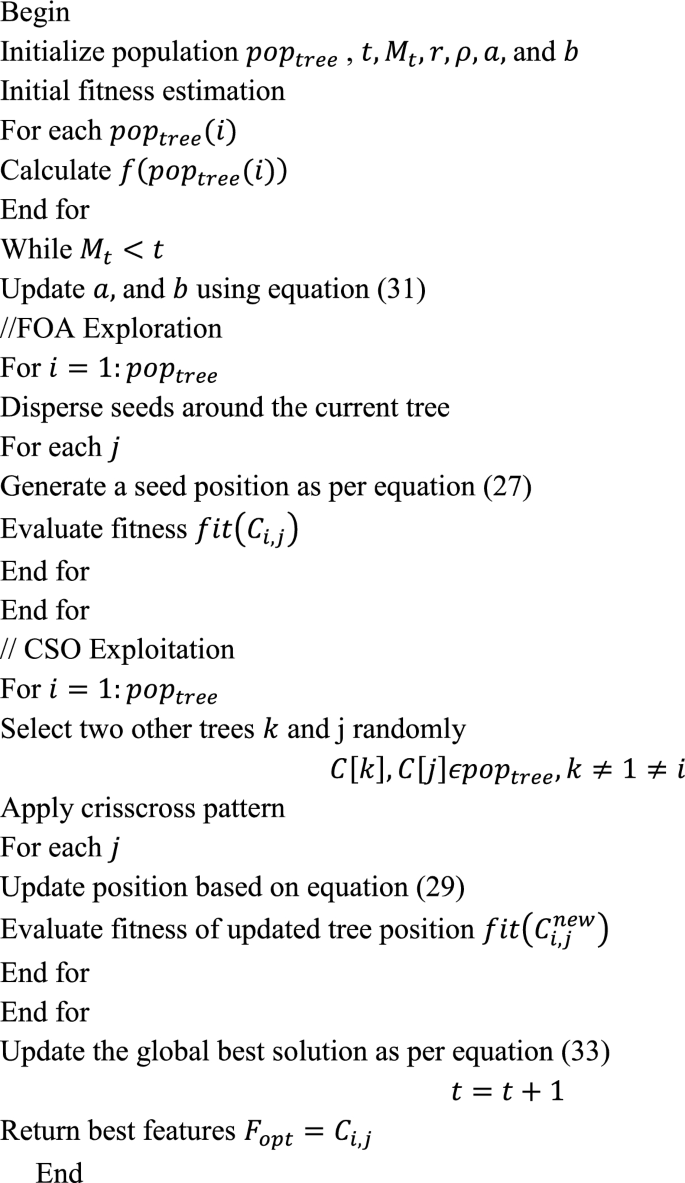
Pseudocode of Developed CSFOA.
ArabSignNet-based detection
A new ArabSignNet using DenseNet-EfficientNet and attention-based Deep ResNet is proposed for enhanced detection. The architecture of the proposed model is shown in Fig. 15.
(3) Hybrid DenseNet and EfficientNet: DenseNet-12141 links every layer to each other layer with a feed-forward fashion. EfficientNet-b042 scales the network’s width, depth, and resolution depend on a compound scaling model, achieving higher accuracy with fewer parameters. The input \({F}_{opt}\) is processed through DenseNet and EfficientNet in parallel to extract diverse and rich feature representations. The features from DenseNet \({F}_{densenet}\left(x\right)\) and EfficientNet \({F}_{efficientnet}\left(x\right)\) are concatenated to form a unified feature map \({F}_{DE}\left(x\right)\) as formulated in Eq. (35), in which \(x\) indicates the input. The architecture of the proposed Hybrid DenseNet and EfficientNet is shown in Figs. 12 and 13, respectively.

Architecture of Hybrid DenseNet and EfficientNet.

Layered architecture of Hybrid DenseNet and EfficientNet.
$${F}_{DE}\left(x\right)=\left[{F}_{densenet}\left(x\right),{F}_{efficientnet}\left(x\right)\right]$$
(35)
(4) Attention-Based Deep ResNet: The optimal features \({F}_{opt}\) is fed into a deep ResNet3 with integrated attention mechanisms. This stage focuses on refining the features by emphasizing the most informative parts of the image as stated in Eq. (36), in which \({F}_{att}\left(x\right)\) indicates attention-weighted feature map, \({\varphi }_{i}\) stands for weights assigned from attention mechanism to different features, and \({F}_{resnet}^{i}\left(x\right)\) addresses feature maps processed by ResNet. The architecture of the model is shown in Fig. 14.
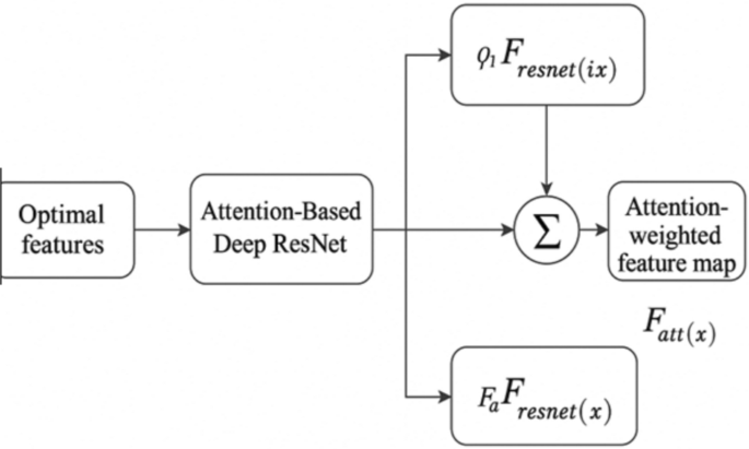
Attention-based deep ResNet.
$${F}_{att}\left(x\right)=\sum_{i} {\varphi }_{i}\cdot {F}_{resnet}^{i}\left(x\right)$$
(36)
This DL-based detection architecture focuses on both accuracy and computational efficiency.
(A) EL with Model Averaging.
An EL approach is implemented by combining the predictions from multiple models such as DenseNet, EfficientNet, and ResNet using model averaging to enhance the final detection accuracy. DenseNet, EfficientNet, and ResNet are trained separately on the same detection task. Each model learns to extract features and make predictions based on its unique architecture. After training, each model generates its prediction for a given input image as \({F}_{DE}\left(x\right)\) and \({F}_{att}\left(x\right)\). The predictions from the three models were combined by a concatenation layer as shown by Eq. (37).
$${F}_{final}\left(x\right)=Concat\left[{F}_{DE}\left(x\right),{F}_{att}\left(x\right)\right]$$
(37)
The final prediction \({F}_{final}\left(x\right)\) is used to make the detection decision. For classification, this involves selecting the class with the highest probability. Each model \({M}_{i}\) outputs a probability distribution over the classes as defined in Eq. (38), in which \({P}_{{M}_{i}}\left(x\right)\) is the final decision.
$${P}_{{M}_{i}}\left(x\right)=softmax\left({F}_{final}\left(x\right)\right)$$
(38)
Table 3 summarizes the hyperparameter settings of suggested method.

