Framework
The research framework of this article is shown in Fig. 1.
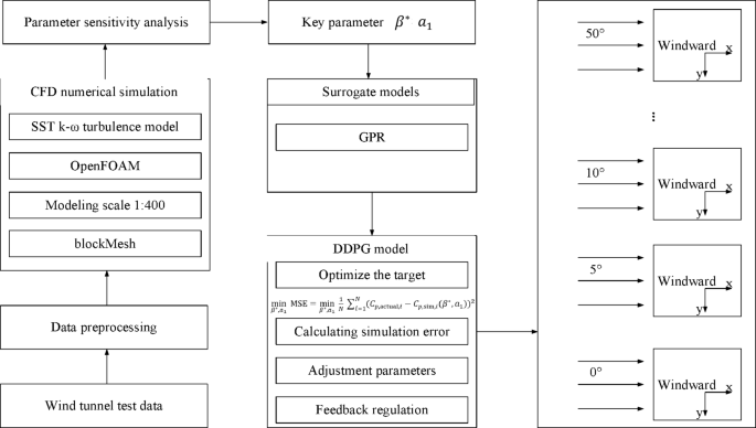
Research framework of this article.
The OpenFOAM is used to implement SST k-ω turbulence model, and boundary conditions, mesh type, quantity, etc., are set. Using the SST k-ω turbulence model, a structured hexahedral mesh was created using blockMesh, with approximately 150,000 cells. The boundary conditions were set as follows: a fixed velocity of 10 m/s at the inlet, zero gradient at the outlet, and no-slip conditions on the wall. The turbulence model is implemented in OpenFOAM, with the inlet velocity set to 10 m/s, the outlet pressure set to zero gradient, and the wall using the noSlip boundary condition. The blockMesh type is used for meshing to ensure calculation accuracy. Sensitivity analysis is conducted on the parameters of the SST k-ω turbulence model to identify key parameters that have a significant impact on the simulation results. A Gaussian process regression model and SVM are established to select the optimal surrogate model. The surrogate model is trained using initial CFD simulation data to approximate the output of the turbulence model.
Analysis of blunt body flow problem: the wind direction angle is set to θ = 0°, and the DDPG algorithm is used for parameter optimization. The optimized parameters are substituted into the SST k-ω turbulence model and validated using wind tunnel test data33,34. Through the exploration and utilization of intelligent agents in simulated environments, model parameters are gradually adjusted to minimize wind pressure simulation errors.
Parameter optimization adaptability analysis: the range of different wind direction angles θ is set within the range of 0° to 50°, and the wind direction angle is adjusted every 5° interval. The optimized parameters are substituted into the SST k-ω turbulence model, and the simulated WPCs are output through the surrogate model. The optimization effect is verified using wind tunnel test data. “Optimization effect” refers to the improvement in the accuracy of the optimized SST k-ω turbulence model in predicting the wind pressure coefficient, including the reduction in MSE, the reduction in RMSE, and the enhanced fit between the optimized model calculation results and the wind tunnel test data. The WPCs under different wind direction angles are compared to evaluate the adaptability and consistency of parameter optimization at each wind direction angle.
In order to ensure data quality, the collected data is cleaned, and abnormal data points are removed. Missing data items are filled in through interpolation to ensure the continuity of the data in time and space. Data cleaning refers to the preprocessing of the collected raw data to improve data quality and reliability. In this study, the identification of abnormal data points is based on statistical analysis methods, mainly using the standard deviation method, that is, calculating the deviation of the data point relative to the mean. If the deviation exceeds three times the standard deviation, it is regarded as an outlier and eliminated. Data cleaning also includes the detection of duplicate data and physically unreasonable data, including negative wind pressure coefficients or flow velocities beyond a reasonable range. For missing data, linear interpolation is used to fill in to ensure the continuity of the data in time and space, thereby improving the calculation accuracy and stability of the turbulence model. Outliers are calculated by comparing the deviation of the data point from the mean to the multiple of the standard deviation, and are considered outliers when the multiple is greater than 3. Missing data is processed by mean filling to ensure the continuity and accuracy of the data and avoid negative impact on model performance.
The deviation between data points and the mean is calculated as a multiple of the standard deviation, using the equation:
$$Z=\frac{X-\stackrel{-}{X}}{\sigma }$$
(1)
In Eq. (1), \(\stackrel{-}{X}\) represents the mean and \(\sigma\) represents the standard deviation. When \(\left|Z\right|>3\), it indicates that the data point is an outlier. The mean here refers to the arithmetic average of all observations in the data set and is used to measure the central tendency of the data. The standardized deviation evaluates the relative position of the data point in the overall distribution by calculating the deviation of the data point from the mean and dividing it by the standard deviation to identify outliers.
The mean of the data is used to fill in missing values, and the equation for the mean of the data is:
$$\stackrel{-}{X}=\frac{{\sum }_{i=1}^{n}{X}_{i}}{n}$$
(2)
The “mean of the data” refers to the arithmetic average of all valid observations in the data set, that is, the sum of all data points divided by the number of data points. The mean is used to fill in missing values to maintain data consistency, reduce information loss, and ensure the stability and accuracy of statistical analysis or model training.
Construction of numerical simulation environment
The inlet velocity is set according to the wind speed in the wind tunnel test, and the outlet pressure is set to atmospheric pressure. The wall conditions need to consider the roughness and non slip conditions of the wind tunnel wall. Through these settings, it is ensured that CFD simulation can accurately reflect the flow field characteristics in wind tunnel tests, thereby improving the reliability and accuracy of simulation results.
The wind tunnel test data used in this article is sourced from the Wind Tunnel Laboratory of Tokyo Institute of Technology in Japan35,36. The building wind load model is shown in Fig. 2.

Building wind load model.
OpenFOAM is used to build building wind load models. In OpenFOAM37,38, the length, height, and width of the model are set to 0.1 m, and the scale of the model modeling is 1:400. The exposure factor is set to \(\frac{1}{4}\). The start time is set to 0s; the end time is set to 32s; the sampling frequency is set to 1000 Hz. The network type is set through blockMesh; the windward and leeward faces are set as patch; the other faces are set as wall. 25 measurement points are arranged on each of the four surfaces of the building. When the wind exerts pressure on the building surface, the value is positive, and when the wind exerts suction on the building surface, the value is negative.
The boundary conditions set by OpenFOAM are shown in Table 1.
In OpenFOAM, nut is a variable representing turbulent viscosity and is used to describe the effects of turbulence. The turbulent kinetic energy equation is expressed as:
$$\frac{\partial k}{\partial t}+{U}_{j}\frac{\partial k}{\partial {x}_{j}}={P}_{k}-{\beta }^{*}k\omega +\frac{\partial }{\partial {x}_{j}}\left[\left(\nu +{\sigma }_{k}{\nu }_{t}\right)\frac{\partial k}{\partial {x}_{j}}\right]$$
(3)
In Eq. (3), k represents turbulent kinetic energy; \({U}_{j}\) is the velocity component; \({\beta }^{*}\) is the turbulent dissipation coefficient; \({P}_{k}\) is the turbulence generation term; \(\omega\) represents the specific dissipation rate; \(\nu\) is the coefficient of motion viscosity; \({\nu }_{t}\) is the turbulent viscosity coefficient; \({\sigma }_{k}\) is the turbulent Prandtl number in the turbulent kinetic energy equation.
The specific dissipation rate equation is expressed as:
$$\frac{\partial \omega }{\partial t}+{U}_{j}\frac{\partial \omega }{\partial {x}_{j}}=\alpha \frac{\omega }{k}{P}_{k}-\beta {\omega }^{2}+\frac{\partial }{\partial {x}_{j}}\left[\left(\nu +{\sigma }_{\omega }{\nu }_{t}\right)\frac{\partial \omega }{\partial {x}_{j}}\right]+2(1-\text{F})\frac{{\sigma }_{\omega 2}}{\omega }\frac{\partial k}{\partial {x}_{j}}\frac{\partial \omega }{\partial {x}_{j}}$$
(4)
In Eq. (4), \(\alpha\) is the coefficient of the turbulence model, which takes different values in different regions and can be represented as \({\alpha }_{k1}\), \({\alpha }_{k2}\), \({\alpha }_{\omega 1}\), and \({\alpha }_{\omega 2}\). \(\beta\) is the coefficient of the turbulence model, which takes different values in different regions and can be represented as \({\beta }_{1}\) and \({\beta }_{2}\). \({\sigma }_{\omega }\) and \({\sigma }_{\omega 2}\) represent the turbulent Prandtl number in the specific dissipation rate equation and the turbulent Prandtl number in the mixing function, respectively.
Production item \({P}_{k}\) is represented as:
$${P}_{k}={\tau }_{ij}\frac{\partial {U}_{i}}{\partial {x}_{j}}$$
(5)
$${\tau }_{ij}=2{\nu }_{t}{S}_{ij}-\frac{2}{3}{\delta }_{ij}k$$
(6)
The turbulent viscosity coefficient \({\nu }_{t}\) is expressed as:
$${\nu }_{t}=\frac{{a}_{1}k}{\text{m}\text{a}\text{x}({a}_{1}\omega ,S{F}_{2})}$$
(7)
In Eq. (7), \({a}_{1}\) is a parameter in the turbulent viscosity coefficient.
S is the modulus of the strain rate tensor:
$$S=\sqrt{2{S}_{ij}{S}_{ij}}$$
(8)
The mixed function F is used to achieve a smooth transition between the k-ω model and the k-\(\in\) model:
$${F}_{1}=\text{t}\text{a}\text{n}\text{h}\bigg({\bigg(\text{m}\text{i}\text{n}\bigg[\text{m}\text{a}\text{x}\bigg(\frac{\sqrt{k}}{{\beta }^{*}\omega y},\frac{500\nu }{{y}^{2}\omega }\bigg),\frac{4{\sigma }_{\omega 2}k}{C{D}_{k\omega }{y}^{2}}\bigg]\bigg)}^{4}\bigg)$$
(9)
$${F}_{2}=\text{t}\text{a}\text{n}\text{h}\bigg({\bigg(\text{m}\text{a}\text{x}\bigg(\frac{2\sqrt{k}}{{\beta }^{*}\omega y},\frac{500\nu }{{y}^{2}\omega }\bigg)\bigg)}^{2}\bigg)$$
(10)
In Eq. (9), \(C{D}_{k}\) is the derivative of turbulent kinetic energy; y is the distance from the wall surface; \({\sigma }_{\omega 2}\) is the turbulent Prandtl number in the dissipation rate equation.
The default values of each parameter in the SST k-ω turbulence model are shown in Table 2.
Parameters \({\beta }_{1}\), \({\beta }_{2}\), and \({\beta }^{*}\) affect the turbulent energy dissipation rate and are crucial for predicting the accuracy of flow separation and reattachment regions. \({a}_{1}\) is used to adjust the behavior of the model in different flow regions to ensure reasonable results can be obtained in both near wall and far wall regions. By optimizing these parameters, the performance of the model in complex flow fields is improved, making it more accurate in simulating fluid separation, reattachment, and vortex phenomena.
The sensitivity analysis was carried out by adjusting the key parameters of the SSTk-ω model (multiplying by 0.6, 1.0, and 1.4), comparing the simulation output errors, and using the Sobol index and grid independence test to quantitatively evaluate the parameter impact, thereby identifying the factors that affect the simulation results and ensuring that the simulation results are accurate and reliable.
The 10 parameters mentioned in Table 2 are subjected to parameter changes, with values of 0.6 and 1.4 times the original parameter values. When the Sobol method is used to evaluate the key parameters of the turbulence model, multiple combinations of parameter space are generated through sampling methods, and then the model output corresponding to each combination is calculated. Using the Sobol index decomposition method, the total variance is decomposed into the main effect and interaction effect of each parameter to quantify the contribution of each parameter to the output variance. By performing sensitivity analysis on multiple turbulence model parameters, the key parameters that have a greater impact on the model prediction accuracy can be identified. The reason why the parameter variation range is chosen to be 0.6 and 1.4 is to simulate the common variation range of turbulence model parameters in actual engineering. This variation range can effectively cover possible errors and uncertainties without deviating too much from the original value, ensuring that the sensitivity analysis can reflect the impact of parameter changes on the simulation results. The average WPCs of each measurement point under different parameters are shown in Fig. 3. Sensitivity analysis evaluates the impact of each parameter on the simulation results by changing the values of the model parameters (0.6 times and 1.4 times). By observing the changes in the average wind pressure coefficient under different parameter settings, key parameters that have a significant impact on the simulation results are identified.

Average WPCs at different measurement points under different parameters. (A) \({\alpha }_{k1}\); (B) \({\alpha }_{k2}\); (C) \({\alpha }_{\omega 1}\) ; (D) \({\alpha }_{\omega 2}\); (E) \({\beta }_{1}\); (F) \({\beta }_{2}\) ; (G) \({\beta }^{*}\); (H) \({a}_{1}\); (I) \({\sigma }_{k}\); (J) \({\sigma }_{\omega }\)
Figure 3 shows the average WPCs of each measurement point under 10 parameter changes in sequence. The significance of the parameter changes on the simulation results can be determined by observing the numerical curve changes of the average WPCs. It can be seen that in the range of measurement points 1–5, 21–25, 41–45, 61–65, 81–85, the measurement points are located on the windward side, and the average WPC is relatively large. On the basis of the default parameter values, 0.6 times the parameter value and 1.4 times the parameter value are also set. By comparing the three curves under each parameter, it can be found that the curves in Fig. 3G and H show the most significant differences between the 0.6 times parameter and the default parameter, as well as between the 1.4 times parameter and the default parameter. Therefore, \({\beta }^{*}\) and \({a}_{1}\) are key parameters that have a significant impact on the simulation results.
Establishment of surrogate model
The surrogate model can quickly approximate complex turbulence phenomena and significantly reduce computational costs by using a small amount of high-precision computational fluid dynamics simulation data for training. Surrogate models can efficiently explore the parameter space, optimize turbulence model parameters, and improve simulation accuracy and reliability. By refining simulation results, accurately predicting and analyzing turbulence behavior can improve computational efficiency in turbulence research and facilitate subsequent parameter optimization analysis. In order to solve the problems of overfitting and generalization of the proxy model, cross-validation and Bayesian optimization can be used to adjust hyperparameters. In addition, the fusion of multi-credibility proxy models improves adaptability, and combined with the online update mechanism, the model dynamically adapts to different turbulence simulation scenarios, improving robustness and generalization ability.
Surrogate models are used for regression tasks. They approximate complex physical processes at low computational cost by learning the mapping relationship between input variables and output results. In turbulence simulation, surrogate models can replace high-cost CFD simulations to achieve efficient parameter optimization.
This article uses Gaussian process regression39,40 and SVM41,42 to establish surrogate models, and compares their data fitting effects to select the optimal surrogate model. GPR and SVM were selected for surrogate model analysis based on their respective advantages: GPR can provide uncertainty quantification, is suitable for small samples and high-dimensional problems, has good generalization ability, and is suitable for parameter optimization in turbulence simulation; SVM performs well in processing high-dimensional nonlinear data, can effectively avoid overfitting, and improve model robustness.
SVM and GPR were selected as surrogate models for comparison, mainly based on their complementary characteristics in regression tasks. GPR has the ability to quantify uncertainty and is suitable for small sample high-dimensional problems, while SVM performs well in dealing with nonlinear relationships and high-dimensional features and can effectively avoid overfitting. By comparing the fitting accuracy of the two, the selection of the optimal surrogate model is verified.
The mean function in Gaussian process regression is represented as:
$$m\left(x\right)=\mathbb{E}\left[f\right(x\left)\right]$$
(11)
The covariance function is expressed as:
$$k(x,{x}^{{\prime }})=\mathbb{E}\left[\right(f\left(x\right)-m\left(x\right)\left)\right(f\left({x}^{{\prime }}\right)-m\left({x}^{{\prime }}\right)\left)\right]$$
(12)
During the training process, the logarithmic marginal likelihood function is maximized to optimize the parameters of the kernel function. The logarithmic marginal likelihood function is:
$$\text{l}\text{o}\text{g}p\left(\mathbf{y}\right|X)=-\frac{1}{2}{\mathbf{y}}^{{\top }}{K}^{-1}\mathbf{y}-\frac{1}{2}\text{l}\text{o}\text{g}|K|-\frac{n}{2}\text{l}\text{o}\text{g}2\pi$$
(13)
The kernel function used in SVM is the radial basis function, and the equation is:
$$k(x,{x}^{{\prime }})=\text{e}\text{x}\text{p}(-\gamma \parallel x-{x}^{{\prime }}{\parallel }^{2})$$
(14)
In Eq. (14), \(\gamma\) is the kernel parameter.
SVM adopts an \(\in -\)insensitive loss function to ignore the deviation of errors within the \(\in\)-range:
$${L}_{\in }(y,f(x\left)\right)=\text{m}\text{a}\text{x}(0,|y-f\left(x\right)|-\in )$$
(15)
The comparison of data fitting effects between GPR and SVM is shown in Fig. 4. SVM and GPR are chosen for comparison because they perform well in dealing with regression problems. SVM can effectively handle high-dimensional data and avoid overfitting, while GPR provides good uncertainty quantification and is suitable for complex nonlinear relationships. Both are often used to balance accuracy and computational efficiency in surrogate model construction, so they are ideal choices for comparison.

Data fitting performance of GPR and SVM. (A) GPR data fitting; (B) SVM data fitting.
Using \({\beta }^{*}\) and \({a}_{1}\) for parameter input, 1000 data simulations are conducted in OpenFOAM. The average WPC is used as the corresponding output data. GPR and SVM are respectively used for data fitting. Comparing Fig. 4A and B, it can be intuitively analyzed that the data fitted by GPR is very close to the generated data in OpenFOAM, while the data fitting effect of SVM is relatively poor. Surrogate models are used for regression tasks and make predictions by learning the relationship between input and output. By approximating the calculation process of the actual model, the computational cost is reduced. Surrogate models perform well in optimization problems and can provide fast approximate solutions for complex systems.
The equation for MSE (Mean Square Error) is:
$$\text{M}\text{S}\text{E}=\frac{1}{n}\sum _{i=1}^{n}({y}_{i}-{\widehat{y}}_{i}{)}^{2}$$
(16)
The equation for the average absolute error is:
$$\text{M}\text{A}\text{E}=\frac{1}{n}\sum _{i=1}^{n}|{y}_{i}-{\widehat{y}}_{i}|$$
(17)
In Eqs. (16) and (17), \({y}_{i}\) and \({\widehat{y}}_{i}\) represent the predicted and actual average WPCs, respectively.
The fitting error results of GPR and SVM models under 10 fold cross validation are shown in Table 3.
The data fitted by GPR and SVM models, as well as the average WPC data output by SST k-ω turbulence model, are analyzed by MSE and MAE. By comparing four sets of data, it can be found that the MSE and MAE of GPR are lower than SVM, with an average MSE of 0.00345 and an average MAE of 0.04883 for GPR; the average MSE of SVM is 0.0196 and the average MAE is 0.05183. Based on the results in Fig. 4; Table 3, GPR can better approximate the output of the SST k-ω turbulence model. Therefore, this article chooses GPR as the surrogate model. Surrogate models can accelerate parameter optimization analysis by approximating complex actual models. Different surrogate models have their own advantages and disadvantages. They may suffer from overfitting problems, resulting in inaccurate predictions of new data. In addition, surrogate models are usually designed for specific situations. When the model settings or parameters change, the original surrogate model may not be able to generalize effectively, reducing its applicability.
The advantage of using the GPR proxy model is that it can efficiently approximate CFD simulation results, significantly reduce computational costs, and provide uncertainty quantification to enhance prediction stability. Compared with direct CFD simulation, GPR can use a small amount of high-precision CFD data for training, reducing computing resource consumption and making parameter optimization more efficient. In addition, GPR has good generalization capabilities and can still accurately fit complex flow field characteristics under small sample conditions, thereby achieving a better balance between computational efficiency and accuracy when optimizing turbulence model parameters.
Application of DDPG algorithm
Reinforcement learning is a machine learning method that learns by interacting with the environment and based on reward signals. Its main components include agents, environments, states, actions, and rewards. Agents interact with the environment by selecting actions to obtain rewards or penalties, thereby optimizing decision-making strategies. In this paper, reinforcement learning is used to optimize the parameters of the turbulence model, and the reward signal is used to guide the model to select the optimal parameters to improve simulation accuracy and computational efficiency.
Reinforcement learning is a self-learning method in which an intelligent agent interacts with the environment and optimizes its strategy based on reward signals. Its key components include state, action, reward, strategy, and value function. This study uses the DDPG algorithm in deep reinforcement learning to optimize the parameters of the SST k-ω turbulence model, where the state represents the initial parameters of the turbulence model, the action corresponds to the parameter adjustment, the reward function aims to minimize the error of the wind pressure coefficient, and the policy network is used to learn the optimal parameter update rules. Compared with traditional optimization methods (such as GA and PSO), DDPG can efficiently search in continuous high-dimensional space, and combine with the GPR agent model to accelerate the optimization process, thereby improving computational efficiency, reducing simulation costs, and improving the applicability and generalization ability of the model.
The action space represents the adjustment values of parameters, and the reward function is defined as a negative simulation error, that is, the optimization objective is to minimize the error and obtain the highest reward.
The Actor network43,44 accepts the current parameter value and outputs an action, which is the parameter adjustment value; the Critic network calculates the reward value obtained after taking this action. By continuously updating the parameters of these two networks, the DDPG algorithm can gradually approach the optimal strategy. The DDPG optimization framework based on the GPR proxy model is shown in Fig. 5.

DDPG optimization framework based on the GPR proxy model.
DDPG is adopted for single wind direction angle optimization, and a fixed sized experience replay pool is initialized to store the interactive data generated during the optimization process. In each training step, a batch of data samples are randomly selected from the experience replay pool for training to reduce bias caused by data correlation. By executing actions (adjusting parameters \({\beta }^{*}\) and \({a}_{1}\)), new states and rewards are obtained. Under a single wind direction angle, by adjusting the parameters, the simulation error of the WPC in the SST k-ω turbulence model is minimized. After each execution of the action, the simulation error is calculated and used as feedback as a reward to guide the next step of parameter adjustment.
The optimization objective is to minimize the simulation error of the WPC in the SST k-ω turbulence model, measured by mean square error. The optimization objective function equation is:
$$\underset{{\beta }^{*},{a}_{1}}{\text{m}\text{i}\text{n}}\text{M}\text{S}\text{E}=\underset{{\beta }^{*},{a}_{1}}{\text{m}\text{i}\text{n}}\frac{1}{N}\sum _{i=1}^{N}({C}_{p,\text{a}\text{c}\text{t}\text{u}\text{a}\text{l},i}-{C}_{p,\text{s}\text{i}\text{m},i}({\beta }^{*},{a}_{1}){)}^{2}$$
(18)
In Eq. 18, \({C}_{p,\text{a}\text{c}\text{t}\text{u}\text{a}\text{l},i}\) and \({C}_{p,\text{s}\text{i}\text{m},i}\) represent the actual and simulated WPCs for the i-th data point, respectively.
The equation for the reward function is:
$$r({\beta }^{*},{a}_{1})=-\frac{1}{N}\sum _{i=1}^{N}({C}_{p,\text{a}\text{c}\text{t}\text{u}\text{a}\text{l},i}-{C}_{p,\text{s}\text{i}\text{m},i}({\beta }^{*},{a}_{1}){)}^{2}$$
(19)
During the optimization process, GPR surrogate models are used to replace costly CFD simulations. The GPR model can quickly predict the simulation error after parameter adjustment and improve optimization efficiency by training the initial CFD simulation data. In each training step, the GPR surrogate model is used to predict simulation errors under different parameter combinations, thereby accelerating the optimization process.
The Adam optimizer dynamically adjusts the learning rate by calculating the moving average of gradients, enabling the network parameters to converge quickly and stably. The Adam optimizer updates the parameters of the Actor and Critic networks based on the samples extracted from the experience replay pool to continuously improve the quality of the strategy.
DDPG is adopted for multi-wind direction angle optimization, with the range of wind direction angle θ set within the range of 0° to 50°, and wind direction angle adjustment conducted every 5° interval. By using data from multiple wind directions, the dataset is expanded to analyze the practical application effects of DDPG optimization.
The calculation of WPC is:
$${C}_{p}=\frac{p-{p}_{{\infty }}}{\frac{1}{2}\rho {V}^{2}}$$
(20)
Software version information
-
Visio: Microsoft Visio 2019, https://www.microsoft.com/zh-cn/microsoft-365/visio/flowchart-software.
-
OpenFOAM: OpenFOAM v2306, https://www.openfoam.com/.
-
Python: Python 3.8, https://www.python.org/.
-
NumPy 1.26.4, https://numpy.org/.
-
Pandas 2.2.2, https://pandas.pydata.org/.
-
Matplotlib 3.8.4, https://matplotlib.org/.
-
SciPy 1.12.0, https://scipy.org/.
-
Scikit-learn 1.4.2, https://scikit-learn.org/.
-
TensorFlow 2.16.1, https://www.tensorflow.org/.
-
PyTorch 2.3.1, https://pytorch.org/.
-
PyFoam 2023.10, https://github.com/PyFoam/PyFoam.
-
Xarray 2024.3.0, https://docs.xarray.dev/.
-
Plotly 5.22.0, https://plotly.com/python/.