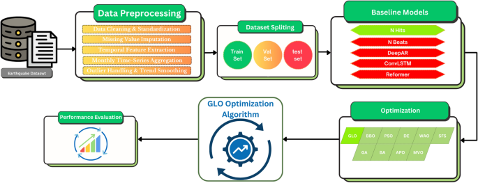
In order to give a concise summary of the proposed experimental setup, the general methodology pipeline used in the current study is summarized in Fig. 1. The data preprocessing of the earthquake data starts with a stage of thorough data preprocessing that consists of structural standardization, analysis of missing values, shaping of time features, categorical cleaning, time-series aggregation, and dealing with outliers. After preprocessing, the data is subdivided into training , testing and validation parts so that it is possible to evaluate the models without bias. A number of deep learning architectures are then used as a basic forecasting model, such as the Neural Hierarchical Interpolation of Time Series (N-HITS), Neural Basis Expansion Analysis of Time Series (N-BEATS), Deep Autoregressive Networks (DeepAR), Convolutional Long Short-Memory (ConvLSTM), and Reformer-based architectures. Several metaheuristic optimization algorithms are being investigated in order to optimize predictive performance and reach an optimal search parameter setting. The main optimization strategy used among them is the Gray Langurs Optimizer Optimization-based Learning Optimizer (GLO), and it is compared with a range of known metaheuristics, Particle Swarm Optimization (PSO), Whale Optimization Algorithm (WOA), Genetic Algorithm (GA), Bat Algorithm (BA), Biogeography-based Optimization (BBO), Differential Evolution (DE), Stochastic Fractal Search (SFS), Arithmetic Optimization (APO), and Multi-Verse Optimization (MVO). Lastly, the models that are optimized are evaluated on the basis of extensive performance appraisal measures in order to ascertain forecasting effectiveness, strength, and ability to generalize.

Overall framework of the proposed seismic time-series forecasting methodology, including data preprocessing, dataset splitting, baseline deep learning models, optimization strategies, and final performance evaluation.
Dataset description
The seismic record, which was used in the study, was acquired by the Government of Canada in Natural Resources Canada (Earthquakes Canada). The catalog is offered via the comma-separated values (csv) format, and this supports scientific computing environments and enables reproducible experimentation. Its time span spans between 1 January 1985 and 1 January 2020, giving a period of over thirty years of documented seismic activity of the Canadian territory and the surrounding areas. Deep time-series forecasting, in particular, is well suited to this extended temporal horizon that allows both learning short-term variations as well as long-term structural dependencies to seismic sequences.
In this study, the forecasting target is defined as the earthquake magnitude recorded in the seismic catalog. Specifically, each observation corresponds to the magnitude value associated with an individual seismic event. Accordingly, the predictive models are designed to estimate future earthquake magnitudes based on historical seismic observations, rather than predicting event counts or occurrence probabilities (Table 2).
The data set is an event level data, and each of the data lines of a table shows an occurrence of an earthquake. Table 1 below, namely tab:dataset features, provides the major features of the dataset. All these properties are the encoders of the temporal, spatial, and geophysical features of seismic events and the basis of built predictive models. As illustrated in Table 21, the latitude range indicates seismic activity stretching further into southern Canada into the high Arctic areas, whereas the longitude distribution is that of the western Pacific margins and eastward intraplate areas. The depths values reveal that most earthquakes are experienced at shallow to intermediate crustal levels, but there are also those that are below 100 km, especially those that are experienced in tectonically active western regions. The magnitude distribution represents the microseismic events that have negative magnitude, which are made possible by sensitive instrumentation networks, and the moderation-to-strong events that extend to magnitude 7.7.
The attribute of magnitude type separates measurement scales of difference, which plays an important part in nurturing constant interpretational coherence spanning seismic records. The location descriptor gives contextual geographic labeling that allows the analysis of regional clustering, whereby the spatial density patterns may be validated qualitatively.
An in-depth statistical analysis of the data shows that there is a great disparity regarding time, magnitude, depth and spatial division.
Trends of the temporal frequencies. The number of events is quite different each year. The previous decades show relatively lower documented rates, and the subsequent years show an increase in the rates of identifying the events, which is probably the result of the improvement in seismic measurement tools and coverage. This is a source of temporal non-stationarity, which underlines the need for models with the capability to represent changing seismic regimes instead of assuming the presence of steady statistical properties.
Magnitude distribution. The magnitude histogram is highly skewed towards the right, with most of the events falling in the low-to-moderate bracket of magnitude (around 0-3). The frequencies of the events decrease quickly with the magnitude, which is in line with the Gutenberg-Richter relationship. This disequilibrium provides a modeling difficulty, whereby infrequent high-magnitude happenings are associated with inappropriate hazard importance and include somewhat restricted training cases.
Depth distribution. The depth histogram shows that the majority of seismic activities are developed in the shallow crustal areas (wholly under 40 km). However, due to the intermediate and deep events, which do go beyond 100 km, there are indicators of multiple seismogenic structures throughout Canadian tectonic provinces. The depth distribution has a multi-modal structure that highlights the significance of keeping depth as a continuum as opposed to discretizing the depth into coarse categories.
Clusters of spatial density. The cluster analysis shows that there is a strong clustering on the western side of Canada, especially on the west of Vancouver Island and British Columbia. Further clusters can also be seen in eastern Canada, such as the Charlevoix Seismic Zone, and scattered activity in the north Arctic. With these spatial density gradients, there is emphasis on tectonic heterogeneity, which provides a reason to incorporate the latitude and longitude directly into the forecasting edifice that can learn spatial influencing scores with a duration negligence.
All in all, the dataset has a good geophysical and geographical variability, extensive temporal coverage and expansive geographic coverage. These qualities render it effective in making deep learning forecasting models and metaheuristic optimization strategies assessment within a consistent national-scale analysis of the seismic.
Data preprocessing
The preprocessing pipeline was developed to make sure that the data is structurally consistent, statistically robust and coherent over time before developing and assessing models. Seismic catalogs are generally heterogeneous in nature, with a combination of continuous geophysical data (e.g., magnitude and depth), spatial (latitude and longitude), and categorical data (e.g., magnitude type and location names). Such heterogeneity, absent from implementing attention to preprocessing, may contain inconsistencies that could sweep forward into model training and worsen its convergence stability, as well as its generalization. Based on that, all preprocessing steps were applied to achieve two complementary goals in a controlled and sequential development: (i) maintain the physical interpretability of seismic observations, and (ii) increase the suitability of data to deep-learning-based time-series forecasting under reproducible experimental conditions.
Dataset Structure Standardization
In order to ensure consistency and clarity throughout all the experimental phases, the raw data schema was refined with semantically explicit conventions of naming the data columns. It is a key step towards reproducibility, and this also avoids ambiguity when the feature engineering, encoding and aggregation are done afterwards. Table 3 shows the final standardized structure. A feature could only be maintained when it contained interpretable information regarding seismic characterization or downstream modeling. Specifically, the temporal attribute (date) should be explicitly named to help the Neo4j database be indexed, time-transformed, and named the geospatial and geophysical variables in a manner that would be compatible with the analysis scripts and modeling libraries.
As demonstrated in Table 3, the column extra was used as an additional field and did not add any consistent or physically significant information to predict. It was thus dropped to eliminate redundancy, much unwanted dimensionality and complete the feature space. This is a structural refinement that enhances the interpretability and also reduces the chances of spurious correlations affecting the learning process.
Missing Value Handling
A missing-value audit was conducted comprehensively to determine completeness on the variables of numerical, categorical and time. It is also essential in seismic catalogs to make sure that missing values are dealt with well because incomplete entries may occur due to instrumentation limitations, late recording or missing standardized metadata formatting.
Primary feature validation was done on essential seismic attributes initially, such as date, latitude, longitude, depth, formation and finally magnitude. These variables constitute the bare possible description of an event. Recordings that had blank values in these fields were reviewed to identify how they would be dropped or rebuilt. There was no deletion that was necessary, and this implies that the primary seismic measurements are very much intact. In numerical variables, any blank records were filled in by the use of n median substitution. Median imputation was chosen as the seismic variables (especially the magnitude and depth) often follow skewness and heavy-tail distributions. It has been seen that the median is a strong central value that is not as sensitive to extreme values and maintains the overall stability of the distribution.
A similar inspection was conducted with categorical variables (mag type, place, province). Mode imputation (the most common class) was used when there were missing values. The decision not to generate artificial rare categories, nor to reject the consistency of encoding, nor to do the same to categories. Upon completion of such procedures, the dataset had a total of 101,365 rows and 0 entries left out. This is critical to deep learning pipelines, whose missing values will raise unstable gradients or implicit bias when treated differently on batches.
Date-Time Conversion and Temporal Feature Engineering
The time-series forecasting depends on temporal coherence. The column date was put in a date type to make it easy to have precise indexing, resampling and temporal windowing. On top of type conversion, temporal decomposition was carried out by taking out year, month, day, and hour. These derived features facilitate the description of multiple-scale temporal interactions, making it possible to make a model learn seasonal variations, inter-annual variability, and possible diurnal reporting biases. Although the ultimate forecasting frequency may be monthly, retaining such decomposed elements enhances the exploratory analysis, helps to check further stratification assumptions and allows aggregation functions to be made consistently.
Province Data Cleaning and Standardization
The feature province offers a regional identifier, which offers spatial stratification and categorical analysis. Any entries in the province that were missing were substituted with unknown to preserve the structural integrity and avoid losing any samples. Moreover, all the province strings were made uppercase in order to remove artificial duplication that is a result of inconsistent casing (e.g. BC vs. bc). This is necessary before arriving at categorical coding because unstandardized labeling may cause irrelevant division of features as well as decreased statistical power.
Monthly Time-Series Aggregation
The raw earthquake is of an event type in which every record is actually a seismic event. In this case, however, the forecasting objective is specified on a time scale that is aggregated. Thus, the data were restructured as a monthly frequency time series by defining resampling of data at a monthly frequency as the index and the monthly event count. Such a transformation is intended to convert irregular event timestamps to a regular time series that can be used in forecasting models based on deep learning, ensuring driving consistency in inputs and outputs in supervised learning.
In order to concentrate on modern seismic activity to decrease historical detection biasness that was related to previous instrumentation and recording methods, time-series modeling only included the records of 2000 and after. The move adds more reliability to the frequency series by highlighting the window during which one can get better catalog completeness and monitoring technology.
Dataset Splitting
The prepared dataset was partitioned into three mutually exclusive subsets to ensure a reliable and unbiased evaluation of the proposed forecasting framework. Specifically, 70% of the data was allocated to the training set, which was used to learn the underlying temporal patterns and model parameters. The remaining data was divided equally between validation (15%) and testing (15%) subsets. The validation set was employed during the training phase to tune hyperparameters and prevent overfitting, enabling the optimization algorithm to guide model selection effectively. The test set, which remained completely unseen during both training and validation, was used exclusively for final performance evaluation to assess the generalization capability of the model. This splitting strategy ensures a balanced trade-off between model learning capacity and robust performance assessment, which is particularly important for non-stationary seismic time-series forecasting.
Because the dataset represents a temporal seismic sequence, the splitting was performed in a chronological time-based manner rather than random sampling. Specifically, earlier observations were assigned to the training set, while more recent observations were reserved for validation and testing. This approach prevents information leakage from future events into past data and provides a more realistic evaluation of forecasting performance in real-world seismic applications.
It is important to emphasize that this strict chronological partitioning ensures temporal consistency and avoids the overly optimistic performance estimates that may arise from random data splitting in time-series forecasting problems. While the current study adopts a fixed train–validation–test split for reproducibility and controlled comparison, more advanced validation strategies such as rolling-origin or walk-forward validation could further assess model robustness under evolving temporal conditions and will be considered in future work.
Smoothing Techniques
Several smoothing techniques were checked on the frequency series of monthly earthquakes to analyse the dynamics of underlying trends and to minimize high-frequency variations. Analytical, not manipulative, is the purpose of smoothing here; whereas a key use of smoothing is to facilitate interpretation of trend structures and volatility regimes, and one purpose of smoothing is to give an indication of the complexity with time with which forecasting models need to be modelled.
Simple moving averages (SMA) of 3, 6, and 12 months were calculated in order to capture the short-run movements, medium-run movements and long-run yearly or regime-wide tendencies. Exponential weighted moving average (EWMA) has also been used to focus on recent data, and that is especially important in those sequences where sudden changes happen, and the sequences have burst reactions. Both trend and variability were considered as a rolling mean, and a rolling standard deviation was calculated to obtain a volatility-sensitive measure of the evolution of seismic frequencies. The Savitzky -Galley filter was also used as it is a good filter to smooth and then to retain the local peaks and troughs, i.e., the filter is essential in preventing artificial suppression of burst-like seismic clusters. Lastly, the elementary change of the percentage was calculated in order to measure month-to-month momentum and volatility movements, in order to enable rapid changes to be detected, which can pose a challenge to forecast stability.
Table 4 summarizes the statistical characteristics of the resulting monthly series. Such values give a quantitative seabed of comprehending variability and justification of the multi-scale forecasting style. According to Table 4 The standard deviation is large with respect to the mean, representing strong month-to-month variability. The wide disparity between maximum and minimum further indicates bursts of seismic events, which is why forecasting models that would help in the analysis of non-linear processes and abrupt regime change, as well as the clustered effects of the time scale, are necessary.
Outlier Detection and Treatment Strategies
There are valid extreme observations included in seismic catalogs, like the large magnitude events or deep earthquakes, which are often not common, but they are physically significant. Therefore, the outlier processing should be done with caution, not to exclude informative phenomena. Instead of comparing the modeling performance with only one outlier treatment, four strategies were considered and used to measure performance sensitivity to extreme-value treatment. The statistical characteristics of every strategy are highlighted in Table 5.
The Winsorized technique limits the extremities of distributions to distributional percentiles, while preserving the whole sample size. The capped strategy limits values to physically realistic values, which maintain the sample size and ensure domain consistency. The removal strategy uses a Z-score with the adjusted Z-score criterion to remove identified extremes and makes the dataset smaller with a change in the dispersion aspects. Testing several strategies is relevant to show strength: in case the predictive performance does not show a significant deviation between these treatments, then the forecasting structure can be said to be less reliant on assumptions of extreme-value preprocessing.
In summary, the preprocessing pipeline will create a clean and standardized dataset that will train a reliable deep learning model. Limiting its phases to schema normalization, robust imputation, temporal feature construction, aggregation to a regular monthly sequence and a systematic outlier strategy assessment results in the pipeline providing a statistically consistent and physically understandable baseline to further forecasting as well as optimization experiments.
Data analysis
On top of the visualization of seismicity (space), we are summarizing the statistics of the magnitude of earthquakes with the use of longitude-based regional division (West, Central, East). With this consolidation, it is possible to have an interpretable comparison of seismic productivity (number of events) and magnitude properties (central tendency and characteristics in the upper-tail using the 95th percentile). The present distance heterogeneity of earthquake occurrence and magnitude distributions. Sometimes, such descriptive statistics can be applied in earthquake catalog studies to describe spatial heterogeneity in the occurrence and magnitude distributions of earthquakes that are based on standardized catalog products (e.g., ComCat) and similar measures of magnitude (e.g., moment magnitude when available) (Table 6). Figure 2 combines two orthogonal spatial representations: (i) a point-based geographic density of events represented by colour-coded magnitude and (ii) a density heatmap of hotspots in seismicity. The explanations presented in the above description find this dual representation important due to its value to highlight both the event-level variability (including magnitude heterogeneity) of information in scattered maps and the clustering and spatial pattern of concentrations in density maps that can be less evident in the immediate point clouds. This combination is consistent with the conventional methods of earthquake catalog data visualization.

Spatial distribution of earthquakes. Left: event locations color-coded by magnitude. Right: earthquake density heatmap identifying hotspots of seismic activity (highest-density cell marked).
One of the fundamental procedures in the process of exploratory seismicity analysis is the quantification of the variation in the earthquake occurrence by the varied aggregation scales. Daily, weekly, monthly, and quarterly reporting counts are the best way to understand the level of activity in the basement (mean rate), whether there can be bursty clustering (maximum) or whether there are quiescent periods (minimum). Such summaries of frequency are a common analysis in catalog-based studies due to their general interpretable description of frequency variability before modeling, as well as being suitable for time-series preprocessing functions like binning and resampling. The U.S. Geological Survey (USGS) ComCatsystem is the common source of event archiving and retrieval in the case of catalog-driven analyses to enable the same temporal indexing and frequency calculations, which are reproducible.
Table 7 summarizes the frequency statistics provided in the frequency table of the frequency statistics into one, thus, all the time scales can be directly compared in this table. The totals are the same on all scales since they represent the same underlying event set, whereas averages and extrema are not the same as the aggregation window. The descriptive results put these temporal plots into context, and allow viewing times when activity is the strongest as being concentrated in the counts of bins and not in catalog size.
Figure 3 plots the same frequency data as a time series at four aggregate levels. The daily panel underlines the high-frequency variability at the moment with short intervals and sharp spikes, but weekly and monthly displays regularize the high-frequency variability and give more focus on the trends on the multi-year scale. The quarterly panel also presents the consistent regime changes and significant clustered periods. Simultaneous demonstration of these resolutions comes in handy when analyzing scale-dependent trends prior to choosing a suitable modeling horizon or making granularity forecasts.

Earthquake frequency time series at daily, weekly, monthly, and quarterly aggregation scales for the analyzed catalog.
To investigate interannual variability with seismics behavior, earthquake magnitudes were summarized in every calendar year from 2005 to 2019. The aggregate per annum gives an understanding of the temporal changes in the central tendency, dispersion and the occurrences of extreme events. These annual summations are common in seismic catalog investigations to evaluate alterations in magnitude distributions and also to observe years that have high seismic energy or greater percent fluctuation.
Table 8 summarizes all annual statistics into a unified table, allowing a direct comparison according to the years. The table gives figures of the number of events, the mean and median magnitude, standard deviation and the lowest and highest magnitude observed per year. The structure enables the identification of the years of high seismic productivity, greater average magnitude, or the abnormally strong intensity events. In Fig. 4, the magnitude distribution during the year was shown using smoothed density profiles. This graph complements the numerical table to show changes in production distribution shape and trend, spread and tail. Those vertical reference lines denote thresholds of magnitude in relation to moderate and strong events, which are easy to interpret in terms of the frequency of larger magnitude events in this or that year.
The combined table and figure of distribution serve as a good analytical view of the interannual seismic variability that portrays several years that have larger magnitude averages or a more divergent distribution.

Distribution of earthquake magnitudes by year (2005–2019). Density curves illustrate annual magnitude variability and highlight moderate and strong magnitude thresholds.
The fundamental features of earthquake-count time series include high variance caused by connected bursting, high-scale structure due to catalog completeness effects, aftershocks association and background-rate variability in the long term. In order to have the strength of the interpretation and later models, it is thus usual to utilize the smoothing and transformation strategies that can reveal the latent trends without having such plausible, diagnostically crucial attributes as peaks, regime change, and volatility. Other methods, used in both time-series analysis and also tweezing methods in other contexts, are moving-average and exponential-smoothing families to remove high-frequency noise, and rolling statistics (e.g., mean with dispersion bands), which measure uncertainty and stability in time. Polynomial-based filters, which include Savitzky-Golay, are frequently used where local extrema are required, and percentage-change transformations will offer a direct representation of momentum and volatility relative to each other. Table 9 summarizes all the descriptions of smoothing techniques, descriptive statistics of the starting monthly series and provides them in one consolidated table. This makes the methodological aspect of each technique recorded along with the underlying scale and variability of data that is necessary in examining the significance of the smoothed trends, as well as the interpretation of the volatility spiking. Figure 5 plots all the smoothing and diagnostic perspectives of the monthly epidemic-frequency series, such as simple moving averages, exponentially weighted moving averages, rolling mean and uncertainty bands, Savitzky-Golay smoothing and the monthly percentage change. The consistent appearance of trends in the shown panel of moving-average and EWM charts suggests cross-techniques validation: trends that are consistent in both charts tend to have a lower likelihood of being created by a specific smoother, whereas the absence of these similarities indicates the existence of on-off spikes of local variability in the percentage-change view that the trend attempts to fit.

Monthly earthquake-frequency smoothing and volatility diagnostics using multiple techniques (SMA, EWM, rolling mean with variability bands, Savitzky–Golay smoothing, and percentage change).
Time series of earthquake counts are often non-stationary and burst-like and misleading this low-level analysis when observed directly in the raw-count space. Deviations relative to (i) the mean over the long term, (ii) a rolling trend estimate, and (iii) a seasonal-adjusted year-over-year (YoY) baseline are more likely to improve quantifying the departures of typical behavior. All these complementary considerations divide absolute anomaly magnitude (mean deviation), short to medium-term irregularity following detrending (rolling-mean deviations) and interannual volatility under placid seasonal positioning (same-month YoY differences). These diagnostics are typically a part of time-series exploratory analysis since they help understand the proportional importance of trend, variability, and episodic shocks before specifying the model. Table 10 summarizes all reported horizon-plot statistic scores into one table, which includes baseline monthly variability (standard deviation and coefficient of variation), detrended variability (standard deviation after subtracting 12 months of rolling mean), and YoY change features (average change, sign balance, extreme differences). The combination of these results allows for a consistent explanation of the fact that the observed instability is either trend-driven, seasonally organized, or contains bursts.
Figure 6 presents these diagnostics as three superimposed deviation panels: (i) deviations relative to the world monthly mean, (ii) deviations relative to the 12 months of rolling means (detrended anomalies), and (iii) year-over-year differences by the same month. Positive deviations mark above-baseline activity, of positive deviations whereas negative deviations mark below-baseline activity. Combination: The panels give a systematic interpretation of the anomalies and make a distinction between long-term departures, trend-adjusted changes, and interannual changes.

Horizon-style deviation diagnostics for monthly earthquake counts (2000–2019): (top) deviation from global mean, (middle) deviation from 12-month rolling mean (detrended), and (bottom) year-over-year differences for the same month.
Extreme or unusual items may be contained in earthquake catalogs either as a result of consciously rare events, reporting bias, location/magnitude bias, or variable network coverage. Since outliers may have a significant effect on descriptive statistics (e.g., mean, variance, kurtosis) in addition to destabilizing data-driven forecasting models, it is natural to compare a variety of outlier-handling methods and measure their effect on both data preservation and distributional regularity. Common methods are winsorization (quantile capping), physically motivated range capping and explicit capping, depending on strong outlier scores (e.g., modified Z-score). These are popular in statistical information preprocessing so as to lessen the power of obsolete values without increasing interpretability.
Table 11 summarizes all the strategy-level statistics into one table, which presents (i) size retention of the data sets, (ii) first-order statistics of the data sets (magnitude, depth, etc.), (iii) higher-order statistical descriptors (skewness, kurtosis, IQR, range), and (iv) quality measures (data-preservation percentage, normality score which is lower with increasing normality). Such a combined perspective provides a clear opportunity to compare the trade-off attained between distributional regularity and not all the observations are saved. Figure 7 visualizes how each strategy alters the empirical distributions of magnitude, depth, latitude, and longitude. Comparing the overlaid histograms clarifies whether a strategy primarily truncates tails (winsorization/capping) or changes sample composition (removal). In particular, the depth panels are informative for diagnosing whether extreme-depth values dominate higher-order moments, while the geographic panels (latitude/longitude) verify that preprocessing does not inadvertently distort spatial coverage.

Comparison of outlier-handling strategies via overlaid distributions for magnitude, depth, latitude, and longitude.
To complement the monthly and quarterly subseries visualizations shown in Fig. 8, all descriptive statistics are consolidated into a single comprehensive table. This unified presentation integrates magnitude and depth statistics across temporal resolutions, enabling direct comparison of central tendency, dispersion, and sample size. The table also highlights seasonal variability patterns, including the most stable and most variable months based on standard deviation of magnitude (Table 12).

Monthly and quarterly subseries plots for earthquake magnitude and depth (1985–2019). Red horizontal bars represent monthly/quarterly means with variability intervals.
All annual magnitude statistics and hourly depth statistics are stacked into one table to supplement the ridgeline visualizations shown in Fig. 9. This consolidated representation allows the investigation of interannual and intraday variability simultaneously, so that the temporal distribution variability at a wide range of scales can be compared (Table 13).

Ridgeline plots illustrating (left) annual magnitude distributions and (right) hourly depth distributions (06:00–21:00). Vertical dashed lines indicate median values within each sub-distribution.
To enhance the interpretability of the proposed predictive framework, SHapley Additive exPlanations (SHAP) were employed to quantify the contribution of each input feature to the model predictions. As illustrated in Fig. 10, the SHAP summary plot presents the relative importance and directional influence of key features in earthquake magnitude forecasting. Features with positive SHAP values increase the predicted magnitude, while negative values reduce it. For example, variables associated with recent seismic activity and higher event frequency tend to increase predictions, reflecting seismic clustering and stress accumulation, whereas features related to lower activity or longer quiescent periods contribute negatively. Furthermore, the spread of SHAP values indicates the strength and variability of feature influence, where wider distributions reflect stronger and nonlinear effects. These results confirm that the model integrates multiple interacting factors rather than relying on a single variable, consistent with the multifactorial nature of seismic processes, and demonstrate that the learned representations capture meaningful geophysical patterns while maintaining model transparency.

SHAP summary plot illustrating the contribution of input features to earthquake magnitude prediction.
Deep learning models
The forecasting model used in the given study combines deep learning architectures that are particularly focused on nonlinear time-series modeling. Sequences of earthquake occurrences have complicated statistical characteristics, such as clustering in time, non-stationary behavior, heavy-tailed magnitude distribution, and bursts of activity. These features require models that can highly characterize hierarchical time structures, long-range dependencies and nonlinear interactions without using restrictive parametric assumptions.
This resulted in the choice of four deep learning structures to evaluate using the baseline on their proven performance with regard to time-series prediction: N-BEATS, DeepAR, ConvLSTM, and Reformer. Moreover, N-HITS was deployed and subsequently chosen as the reference architecture for metaheuristic optimization, because of its better baseline performance and theoretical applicability of multi-scale forecasting to it.
N-BEATS
N-BEATS is a residual deep architecture that is specifically formulated to learn engaging time-series prediction featured by interpretability. It is trained in the function of blocks of stacked fully connected layers organized in forward and backward residual blocks. Every block is taught a basis expansion, which breaks the input signal down into trend and seasonality terms47. In contrast to recurrent or convolutional networks, N-BEATS only consists of deep fully connected layers, which makes it easy to build architecturally, but also allows it to express complex functions.
The residual stacking scheme enables a more and more exact forecast to be refined, which means that there is a falsification of redundancy among the blocks. This format is especially beneficial to seismic frequency information, where decomposition of temporal patterns on a hierarchy basis, e.g., seasonal changes or long-term tectonic movement, can be used to make the information more interpretable and predictive.
DeepAR
DeepAR is a recurrent neural network based on probabilistic forecasting of time- stanza and is designed as an autoregressive. It uses recursive units as the unit of modeling of sequential dependencies, and at the same time approximates parameters of a predictive probability distribution. DeepAR is autoregressive, which means that past observations directly affect the occurrence of future predictions, but the forecast has continuity in time48.
DeepAR can also be described probabilistically, which makes the approach especially useful in seismic forecasting, where quantification of uncertainty is of paramount importance because earthquake of occurrence is a stochastic process. DeepAR is used to predict variation of monthly patterns of seismic frequencies and magnitude through learning conditional distributions instead of deterministic point forecasts. Nonetheless, recurrent architectures can be faced with constraints when representing an extremely long dependency scale when compared to a hierarchical or attention-based architecture.
ConvLSTM
ConvLSTM is based on the traditional Long Short-term memory model but adds convolutional operations into the recurrent gating model. This design allows the modeling of spatial and temporal correlations at the same time. On the data that consists of geographic coordinates of the earthquakes, ConvLSTM has the advantage of showing the spatial locality via convolutional kernels while preserving recurrence in a sequence49.
ConvLSTM has the potential of learning localized spatiotemporal interactions in the Canadian seismic context, where spatial clustering is clear along tectonic edges and intraplate regions. However, convolutional recurrent models might not be scalable in scenarios where there is a requirement to model long-term horizons without hierarchical decomposition mechanisms.
Reformer
Reformer is a transformer architecture that aims to solve the quadratic nature of self-attention mechanisms of traditional systems in terms of their computational complexity. Reformer is able to use a locality-sensitive hashing of approximate attention and reversible layers of the residual (severely limiting the memory usage) and does not require maintaining long-range dependencies50.
Attention-based models should be sufficiently well to represent global temporal interactions, which can potentially be due to the delayed stress redistribution. Transformer architectures may, however, be expensive in both data and hyperparameter optimization to converge with permanently unstable sequences like time series of earthquake frequencies.
N-HITS
The N-HITS (Neural Hierarchical Interpolation for Time Series Forecasting) model was proposed as a hierarchical extension of the N-BEATS framework, with the objective of improving the efficiency of learning multi-scale temporal representations and long-horizon forecasting. Its design is based on hierarchical signal decomposition, allowing the model to capture both coarse-grained and fine-grained temporal dynamics within a unified architecture51.
The architecture consists of multiple hierarchical blocks, where each block is responsible for learning temporal patterns at a specific level of granularity. At the block level, the transformation from input to output can be expressed as:
$$\begin{aligned} y_{\textrm{out}}=\textrm{Block}(y_{\textrm{in}})=\textrm{ReLU}(W\cdot y_{\textrm{in}}+b) \end{aligned}$$
(1)
where \(y_{\textrm{in}}\) and \(y_{\textrm{out}}\) denote the input and output of a block, respectively, W represents the learnable weight parameters, and b is the bias term. This formulation shows that each block performs a nonlinear transformation of the input signal in order to extract informative temporal features.
The hierarchical nature of N-HITS can be understood through a decomposition of the original time series into multiple signal levels and a residual term:
$$\begin{aligned} Y=\sum _{l=1}^{L} S_l + R \end{aligned}$$
(2)
where Y is the original time series, \(S_l\) represents the signal captured at level l of the decomposition, and R is the residual component. This representation reflects the principle that different levels of the architecture specialize in modeling distinct temporal structures of the series.
At each hierarchical level, the corresponding block processes its assigned component independently. The output of the block at level l is written as:
$$\begin{aligned} y_{\textrm{out},l}=\textrm{Block}_l(y_{\textrm{in},l})=\textrm{ReLU}(W_l\cdot y_{\textrm{in},l}+b_l) \end{aligned}$$
(3)
where \(y_{\textrm{in},l}\) and \(y_{\textrm{out},l}\) are the input and output at level l, while \(W_l\) and \(b_l\) denote the trainable parameters associated with that level. In this way, each block focuses on a particular portion of the time series and contributes to the overall hierarchical representation.
This hierarchical structure is particularly suitable for seismic frequency time series, which often exhibit complex non-stationary behavior across multiple temporal scales. For example, long-term tectonic trends and short-term seismic bursts may be captured at different hierarchical levels, improving the model’s ability to represent temporal variability more effectively.
To ensure a fair comparison among the five forecasting architectures considered in this study, namely N-BEATS, DeepAR, ConvLSTM, Reformer, and N-HITS, all models were implemented using the same preprocessing strategy and standardized training conditions. Following baseline experimentation, N-HITS demonstrated stronger predictive stability and a more effective representation of seismic temporal patterns than the alternative architectures.
Accordingly, N-HITS was selected as the reference model for the second-stage metaheuristic optimization process. In that stage, only the hyperparameters of N-HITS were optimized using state-of-the-art metaheuristic algorithms, thereby isolating the contribution of the optimization procedure while preserving architectural consistency.
The inclusion of different forecasting paradigms, including residual architectures, autoregressive recurrent models, convolutional-recurrent hybrids, and transformer-based attention models, provides a comprehensive benchmarking framework. This systematic comparison enables a rigorous assessment of how architectural design influences earthquake forecasting performance before and after the application of advanced optimization strategies.
Metaheuristic optimization
Deep learning models like N-HITS are also rich in terms of representational ability, but their predictive capability is extremely sensitive to the hyperparameter settings. Hyperparameters are used to define the structural complexity and learning dynamics of the net before training, unlike model weights, which are learned using gradient-based backpropagation. Misuse of these parameters can all result in under-fitting, over-fitting, unsteady convergence or poor learning in the case of hierarchical architectures. As a result of this, we need systematic hyperparameter optimization to be able to take advantage of the full modeling capabilities of N-HITS in seismic time-series prediction.
The formalization to search the hyperparameter search space in an adaptive and structured way, therefore, used metaheuristic optimization algorithms. These algorithms utilize the population-based search methods that refine candidate solutions correspondingly based on a given fitness function. The visibility of local refinement (exploitation) over global search (exploration) enables metaheuristics to be an effective exploration technique (boosting nearest neighbor score) at navigating the very nonlinear and multimodal environment of hyperparameters of deep learning solutions.
Metaheuristic algorithms have become strong optimization methods in complex, high-dimensional search spaces in which standard deterministic or gradient-based methods might be ineffective. Both the feature selection and the hyperparameter optimization are combinatorial and nonlinear optimization problems in the seismic forecasting context. The uneven spread of the seismic variables, which can be multicollinear features, and the non-stationarity of the time dynamics contribute to the complexity of these tasks even more. The population-based metaheuristic approaches, therefore, give a flexible and adaptive alternative that can explore such hostile search landscapes.
Role of metaheuristics in feature selection
The importance of feature selection is to achieve better predictive power, less important computational cost, and easier interpretation. In earthquake forecasting data, the number of features can not be very high, but during the process of interaction between spatial, temporal, and geophysical characteristics, redundancy and noise can emerge. The use of a good subset of features will mean that only informative patterns are captured by the model, and not accidental correlations.
Binary metaheuristic algorithms are most appropriately applied to feature selection problems as these algorithms work in discrete search spaces, whereby each candidate solution is a binary vector indicating the choice of a feature (1) or its rejection (0). The natural Selection of subsets- Combinatorics lends itself to this representation. In contrast to greedy or threshold-based methods of filters, binary metaheuristics are used to assess the feature subsets in their entirety within a fitness function, which frequently carries predictive error and subset size evaluations jointly. Such a multi-guide to adequate ensuring that the algorithm optimizes dimensionality reduction reflects the predictor.
In comparison with standard filtering techniques (e.g., correlation-based ranking, mutual information), using metaheuristic-based feature selection takes into consideration the inter-feature correlations instead of trying to consider each feature in isolation. Filter methods can be calculated very fast, yet can not resolve nonlinear interactions, which are key in seismic time-series modeling. The embedded techniques include feature selection in training the model, e.g., L1-regularized regression, or importance ranking methods based on trees. Although effective in some sense, embedded approaches are usually bound to a particular model architecture and are unlikely to be more broadly applicable than that architecture.
By contrast, metaheuristic feature selection is model-agnostic, and it can optimize a subset of features directly in terms of a desired predictive goal. This can be especially beneficial in the case of nonlinear deep learning models, in which the features can be viewed as uninterpretable, and their importance can be readily noted. Dimensional reduction with preservation of predictive ability makes binary metaheuristics more cost-effect to compute and curb overfitting, as well as enhances the predictability of seismic forecasting models.
Role of metaheuristics in model optimization
In addition to the aspects of feature selection, metaheuristics are the main component in the optimization of hyperparameters in deep learning models. Learning rate, network depth, batch size, regularization coefficients and architectural configurations are hyperparameters that play a significant role in determining the training dynamics and ultimate predictive accuracy. The space of hyperparameters is usually, however, large, nonlinear, and in part discrete, resulting in exhaustive search being computationally infeasible.
Metaheuristic optimization is a mechanism giving adaptive space exploration. Search strategies can be applied based on the population, which has the benefit of simultaneously evaluating many candidate configurations, which is more likely to break local minima and find solutions that are competitive on a global scale. Metaheuristics have a greater ability to converge in comparison with grid search or random search approaches, in which sampling patterns are established beforehand.
The role of hyperparameter optimization in deep learning-based seismic forecasting is that it has a direct effect on the convergence time, generalization, and training stability. Correctly tuned learning rates eliminate gradient explosion or vanishing effect, whereas regularization parameters are tuned to decrease overfitting in swamp seismic sequences. Also, balanced architectural parameters contribute towards the higher capacity of the model to support multi-scale temporal patterns without dragging the irrelevant complexity into the model.
One more significant benefit of metaheuristic optimization is the strength, in other words, robustness. It has the ability to search through a set of solutions to find out, at least by a few folds or validation splits of a problem, which of their specific configurations can resist slight changes in the training data. This increases reduced variance and higher reproducibility, which are the key to working seismic hazard monitoring systems.
In general, the metaheuristic techniques have been used as smart search tools that supplement deep learning structures. When applied to earthquake forecasting, they facilitate the systematic control of dimension and hyperparameter-refinement, which eventually leads to predictive reliability and efficiency.
The selection of the Gray Langurs Optimizer (GLO) in this study is motivated by its suitability for the hyperparameter optimization landscape associated with deep learning-based seismic forecasting models. Although several metaheuristic algorithms such as Particle Swarm Optimization (PSO), Genetic Algorithms (GA), Bat Algorithm (BA), Biogeography-Based Optimization (BBO), and Multiverse Optimization (MVO) have been widely applied in similar contexts, their performance can be limited by premature convergence and reduced population diversity when dealing with high-dimensional and non-convex search spaces.
In contrast, GLO introduces a hierarchical population structure combined with an adaptive role-based search mechanism, which enhances both global exploration and local exploitation. Unlike conventional algorithms that rely on uniform update strategies, GLO employs coordinated movement behaviors, including leader-guided updates, stochastic perturbation, and migration, allowing it to maintain diversity while refining promising solutions. These properties are particularly important for optimizing deep neural networks, where multiple interacting hyperparameters create a complex and highly nonlinear optimization landscape.
Furthermore, GLO demonstrates improved convergence stability and reduced sensitivity to initialization, which are critical for ensuring consistent performance across repeated runs. For these reasons, GLO is selected as the primary optimization algorithm in this study, while other metaheuristic methods are included as benchmark baselines to enable a fair and comprehensive comparative evaluation under identical experimental conditions.
Gray Langurs optimizer (GLO): mathematical formulation and algorithmic structure
Gray Langur Optimizer (GLO) is a metaheuristic population-based implementation that an imitation of the social structure and social foraging behavior of the gray langur groups. The algorithm replicates group interactions governed by hierarchies, where the role of people is determined by the hierarchical structure (alpha, male, female and child), leadership authority, adaptive searching behavior and migration52.
Let N denote the population size and mt the maximum number of iterations. Each candidate solution \(\textbf{X}_i \in {\mathbb {R}}^d\) represents a hyperparameter vector \(\varvec{\theta }\) for N-HITS. The fitness of each individual is evaluated using the validation loss . The best solution found so far is denoted by \(\textbf{X}_{GB}\) with fitness value \(F_{GB}\).
Population Initialization
At iteration \(t=0\), gray langurs are randomly distributed within the predefined search space:
$$\begin{aligned} \textbf{X}_i^{0} = \textbf{X}_{\min } + r_i \odot (\textbf{X}_{\max } – \textbf{X}_{\min }), \end{aligned}$$
(4)
where \(r_i\) is a random vector uniformly distributed in \([0,1]^d\), and \(\odot\) denotes element-wise multiplication.
Hierarchical Division
The population is sorted based on fitness and divided into three main groups:
-
One-male group
-
Multi-male group
-
All-male group
Within each group, individuals are assigned roles (alpha, male, female, child) according to fitness ranking.
Alpha Position Update
The alpha langur (best individual within a group) updates its position toward the global best using:
$$\begin{aligned} \textbf{X}_{\alpha }^{t+1} = \textbf{X}_{\alpha }^{t} + A \cdot (\textbf{X}_{GB}^{t} – \textbf{X}_{\alpha }^{t}), \end{aligned}$$
(5)
where A is an adaptive coefficient controlling exploitation intensity.
Male Position Update
Male individuals update their positions based on dominance interaction:
$$\begin{aligned} \textbf{X}_{m}^{t+1} = \textbf{X}_{m}^{t} + B \cdot (\textbf{X}_{\alpha }^{t} – \textbf{X}_{m}^{t}), \end{aligned}$$
(6)
where B regulates convergence toward the alpha solution.
Female Position Update
Female langurs explore around the alpha using stochastic perturbation:
$$\begin{aligned} \textbf{X}_{f}^{t+1} = \textbf{X}_{\alpha }^{t} + C \cdot \textbf{R}, \end{aligned}$$
(7)
where C is a scaling factor and \(\textbf{R}\) is a random vector promoting exploration.
Child Position Update
Child individuals perform broader exploratory movements:
$$\begin{aligned} \textbf{X}_{c}^{t+1} = \textbf{X}_{c}^{t} + D \cdot (\textbf{X}_{\alpha }^{t} – \textbf{X}_{c}^{t}) + E \cdot \textbf{R}, \end{aligned}$$
(8)
where D and E balance guided exploitation and random exploration.
Autonomy Mechanism
GLO incorporates an autonomy phase in which all individuals may independently update positions using:
$$\begin{aligned} \textbf{X}_i^{t+1} = \textbf{X}_i^{t} + \omega \cdot (\textbf{X}_{GB}^{t} – \textbf{X}_i^{t}), \end{aligned}$$
(9)
where \(\omega\) controls adaptive convergence pressure.
Migration Strategy
To prevent premature convergence, a migration operator is applied based on dynamic parameters \(\omega\) and \(\varphi\):
$$\begin{aligned} \textbf{X}_i^{t+1} = \textbf{X}_i^{t} + \varphi \cdot (\textbf{X}_j^{t} – \textbf{X}_i^{t}), \end{aligned}$$
(10)
where \(\textbf{X}_j\) is a randomly selected individual, and \(\varphi\) determines migration intensity.
Greedy Selection
After each update, feasibility constraints are enforced and fitness is recalculated. A greedy selection mechanism retains improved solutions:
$$\begin{aligned} \textbf{X}_i^{t+1} = {\left\{ \begin{array}{ll} \textbf{X}_i^{t+1}, & \text {if } F(\textbf{X}_i^{t+1}) < F(\textbf{X}_i^{t}), \\ \textbf{X}_i^{t}, & \text {otherwise}. \end{array}\right. } .\end{aligned}$$
(11)
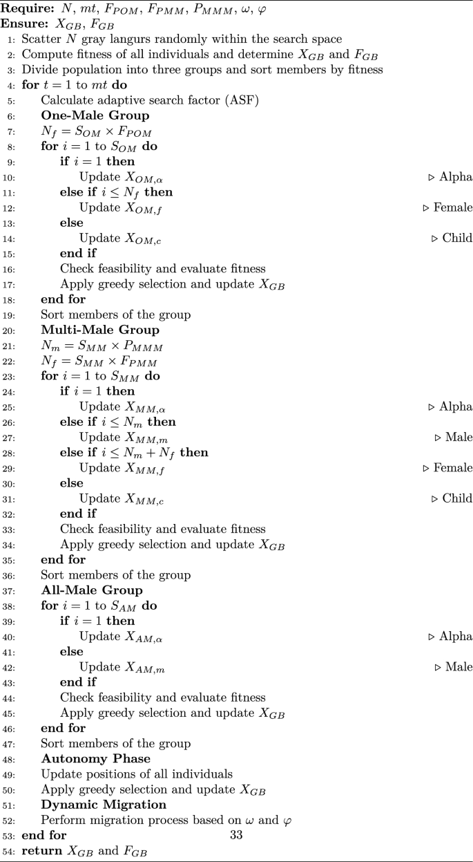
The algorithm iterates until \(t = mt\), at which point the global best solution \(\textbf{X}_{GB}\) and its fitness \(F_{GB}\) are returned. The structured workflow of GLO is formally presented in Algorithm 1. The procedure begins with random initialization of the gray langur population within the predefined search space. After computing the fitness of all individuals and identifying the global best solution \((X_{GB}, F_{GB})\), the population is divided into hierarchical groups. Iterative updates are then performed for the one-male, multi-male, and all-male groups. At each stage, feasibility checks and greedy selection ensure that only improved candidate solutions are retained. Autonomy and migration mechanisms are applied dynamically to enhance exploration and prevent premature convergence. The algorithm terminates after reaching the maximum number of iterations and returns the best solution discovered.
Problem formulation and hyperparameter optimization setup
This subsection formally defines the seismic time-series forecasting problem, the N-HITS forecasting function, the hyperparameter search space, and the GLO-based optimization objective. Let the preprocessed seismic time series be represented as
$$\begin{aligned} {\mathcal {Y}}=\{y_t\}_{t=1}^{T}, \end{aligned}$$
(12)
where \(y_t\) denotes the forecasting target at time step \(t\), and \(T\) is the total number of time-indexed observations after preprocessing. Given a lookback window of length \(L\) and a forecasting horizon \(H\), the input sequence is defined as
$$\begin{aligned} \textbf{x}_t=[y_{t-L+1},y_{t-L+2},\ldots ,y_t], \end{aligned}$$
(13)
and the corresponding future target sequence is defined as
$$\begin{aligned} \textbf{y}_{t+1:t+H}=[y_{t+1},y_{t+2},\ldots ,y_{t+H}]. \end{aligned}$$
(14)
Accordingly, the forecasting task is to learn a nonlinear mapping from the historical input window \(\textbf{x}_t\) to the future seismic target sequence \(\textbf{y}_{t+1:t+H}\).
In the proposed framework, this mapping is modeled using N-HITS as
$$\begin{aligned} \hat{\textbf{y}}_{t+1:t+H} = f_{\mathrm {N\text {-}HITS}}(\textbf{x}_t;\varvec{\theta },\varvec{\lambda }), \end{aligned}$$
(15)
where \(\hat{\textbf{y}}_{t+1:t+H}\) is the predicted output sequence, \(f_{\textrm{N}\text {-}\textrm{HITS}}\) denotes the N-HITS forecasting function, \(\varvec{\theta }\) represents the trainable network parameters learned during model training, and \(\varvec{\lambda }\) represents the hyperparameter configuration optimized by GLO.
The hyperparameter vector is defined as
$$\begin{aligned} \varvec{\lambda } = (L,n_s,n_b,n_l,\textbf{q},u,B,\eta ,\rho ,S,a,r,\omega ,\gamma ,p) \in \Lambda , \end{aligned}$$
(16)
where \(L\) is the input size, \(n_s\) is the number of stacks, \(n_b\) is the number of blocks, \(n_l\) is the number of layers, \(\textbf{q}\) is the frequency downsampling configuration, \(u\) is the number of hidden units, \(B\) is the batch size, \(\eta\) is the learning rate, \(\rho\) is the dropout rate, \(S\) is the maximum number of training steps, \(a\) is the activation function \(r\) is the interpolation mode, \(\omega\) is the weight-decay coefficient, \(\gamma\) is the learning-rate decay factor, \(p\) is the pooling mode, and \(\Lambda\) denotes the predefined mixed discrete-continuous search space reported in Table 14.
The need to ensure reliable data-driven seismic forecasting requires reproducibility and transparency in methodology, especially when model performance is influenced by both architectural design and optimization stability. Therefore, the complete range of N-HITS hyperparameters tested in this work, along with the final configuration selected after optimization, is reported in Table 14. Simultaneously, the structure of the Gray Langurs Optimizer (GLO) is described in Table 15 to clarify the adopted search protocol, convergence controls, and evaluation strategy.
The hyperparameter search was designed within a restricted and interpretable space, following best practices in deep time-series forecasting. Discrete ranges were defined for architectural parameters, including the number of stacks, number of blocks, and number of layers, whereas continuous ranges were used for training and regularization parameters, including the learning rate, dropout rate, weight decay, and learning-rate decay. This structure ensures that the optimization process remains computationally feasible and scientifically interpretable, rather than searching through an unconstrained space that may generate unstable or impractical model configurations.
Table 14 summarizes the N-HITS hyperparameter domains and the final selected values. The selected configuration reflects a balance between representational capacity and regularization strength. Specifically, the lookback window, represented by \(L\) or input_size, determines the temporal context available to the model. The hierarchical depth parameters, including \(n_s\), \(n_b\), and \(n_l\), control the expressive capacity of the decomposition process, allowing the architecture to distribute learning across multiple levels rather than relying on a single temporal scale. The downsampling configuration \(\textbf{q}\) further supports multi-scale modeling by organizing the temporal resolutions used across the N-HITS stacks.
During training, the learning and regularization parameters were optimized to support convergence stability and generalization. The selected batch size balances gradient stability and computational throughput. The learning rate \(\eta\) and learning-rate decay \(\gamma\) control the speed of parameter updates, which is particularly important for non-stationary seismic signals with abrupt temporal variations. The dropout rate \(\rho\) and weight-decay coefficient \(\omega\) reduce overfitting and improve robustness to temporal variability. Finally, the selected activation, interpolation, and pooling settings support stable nonlinear transformation and hierarchical signal reconstruction.
For each candidate hyperparameter configuration \(\varvec{\lambda }\), the model parameters \(\varvec{\theta }\) are trained on the training subset, and the resulting validation error is used as the fitness value. The GLO-based hyperparameter optimization task is therefore formulated as
$$\begin{aligned} \varvec{\lambda }^{*} = \arg \min _{\varvec{\lambda }\in \Lambda } J(\varvec{\lambda }), \end{aligned}$$
(17)
where \(J(\varvec{\lambda })\) denotes the validation-based objective function. Since five-fold cross-validation is used during optimization, the objective function is computed as
$$\begin{aligned} J(\varvec{\lambda }) = \frac{1}{K} \sum _{k=1}^{K} \textrm{MSE}_{\textrm{val}}^{(k)}(\varvec{\lambda }), \qquad K=5, \end{aligned}$$
(18)
where \(\textrm{MSE}_{\textrm{val}}^{(k)}(\varvec{\lambda })\) is the validation mean squared error obtained in the \(k\) -th fold using the N-HITS model configured with \(\varvec{\lambda }\). Thus, GLO searches the predefined hyperparameter space \(\Lambda\) to identify the optimal configuration \(\varvec{\lambda }^{*}\) that minimizes the average validation MSE. The final optimized forecasting model is expressed as
$$\begin{aligned} \hat{\textbf{y}}_{t+1:t+H} = f_{\textrm{N}\text {-}\textrm{HITS}}(\textbf{x}_t;\varvec{\theta }^{*},\varvec{\lambda }^{*}). \end{aligned}$$
(19)
Although Table 14 specifies the model configuration, the effectiveness of the resulting selection depends strongly on the optimization process by which the hyperparameter space is explored. Deep-learning hyperparameter spaces are nonlinear, mixed discrete-continuous, and usually contain multiple local minima. Therefore, population-based optimization is used to improve the probability of identifying effective configurations while maintaining convergence stability.
Gray Langurs Optimizer was configured to provide sufficient exploration of the hyperparameter space while maintaining controlled exploitation around promising configurations. The complete optimization setup is reported in Table 15. A population of 25 agents was used to ensure search diversity while keeping computational requirements manageable. The optimization was executed for 100 iterations, resulting in 2,500 objective evaluations. The objective function was defined as the validation-fold MSE so that the optimizer emphasizes generalization performance rather than training-set fit. In addition, a five-fold cross-validation strategy was adopted to reduce sensitivity to a single validation split and improve the robustness of the fitness estimate.
The initial population was generated using Latin Hypercube Sampling (LHS), which provides broad and stratified coverage of the search space at the beginning of the optimization process. This is particularly useful in seismic forecasting tasks, where model performance can be sensitive to initial hyperparameter choices. The convergence criterion was based on the change in fitness across successive iterations, allowing the optimization process to terminate when no meaningful improvement was observed while avoiding unnecessary additional computation.
Overall, this formulation explicitly connects the seismic input-output forecasting task, the N-HITS forecasting function, the hyperparameter search space, and the GLO-based optimization objective. Together, Tables 14 and 15 provide a complete and reproducible description of the optimized forecasting model and the adopted optimization procedure, supporting transparent comparison with future optimization-aware deep learning pipelines for seismic time-series prediction.
Benchmark algorithms
In order to strictly assess the performance of the proposed GLO, nine well-developed metaheuristic optimization techniques were chosen as benchmark methods. These optimizers’ paradigm will include a variety of methodological paradigms such as swarm intelligence, evolutionary computation, physics-inspired search methods and stochastic diffusion mechanisms. The results were generated with all algorithms having the same population sizes, hyperparameter search scales, and termination requirements in order to be fairly methodological. All optimizers were to be used with the validation loss as the fitness function.
PSO is a swarm-based optimization algorithm that is based on the flocking patterns observed in fish schools and bird flocks. All of these particles are considered to be a candidate solution and modify their movement depending on their previous greatest experience and the greatest solution observed over the swarm. It is also known that PSO converges very fast and is simple, albeit it tends to premature convergence in search spaces characterized by a high multitude53.
WOA emulates the hunting of humpback whales with their bubble-net. It switches between a surrounding of the current optimal solution and the spiral shape search patterns of the area. The adaptive exploration/exploitation enables the WOA to weigh changing global and local search, thus it is applicable to the nonlinear optimization problem54.
GA It is an algorithm in evolutionary computing that is based on natural selection and hereditary principles. There are selection, crossover and mutation operators used to evolve candidate solutions generations by generations. Solutions of high quality will most probably transmit their properties to the next generations, whereas mutation will promote diversity aimed at preventing stagnation. The popularity of GA is based on its strength and the capacity to operate in both continuous and discrete search spaces55.
BA is based on echolocation by bats. It actively modulates the frequency, loudness and pulse rate of emission parameters in order to regulate the switch between the exploration and exploitation phases. The adaptive aspect of BA is making it sharpens search around promising solution when keeping the ability to explore the whole world56.
BBO is a model that is used to describe the migration of species across habitats. The candidate solutions correspond to each habitat with its suitability index, and information exchange is via probabilistic migration. Habitats of high-quality have characteristics of low-quality habitats, which facilitate stable convergence and maintain diversity of the population57.
DE is an evolutionary population-based optimizer based on the differentiation mutation and recombination approaches. It produces candidate solutions which are generated by mixing weighted differing amongst randomly selected persons. DE has been known to be robust and perform well in continuous optimization problems having complicated landscape58.
SFS is based on fractal diffusion. It combines local search based on diffusion and stochastic updating processes in order to improve exploration in many-modal spaces. The fractal character of the search increases the coverage of the search space, as well as minimizing the possibility of local entrapment59.
APO is based on adaptive foraging and interaction behaviour of protozoa. It simulates the competitive and cooperative movement strategies in individuals, and then it actively adapts search directions due to the feedback of the environmental situation. ApO gives priority to adaptive step sizes so as to strike the right balance between convergence and diversity exploration60.
MVO is premised on cosmological ideas like wormholes, white holes, and black holes. In candidate solutions, the exchange of information occurs randomly, and there are extra operators that enhance searching around a solution that is performing well. Early iterations are defined by intense exploration throughout the globe, and later steps are defined by refined exploitation of MVO61.
This framework of benchmark suites offloads the capacity to test the optimization performance of GLO in the process of optimizing the hyperparameters of the N-HITS of the forecasting structure by including swarm intelligence, evolutionary measures, cosmological models and biologically inspired mechanisms into a single experimental framework.
Evaluation metrics
In order to make the assessment of the performance of the forecasting operation rigorous and statistically transparent, several evaluation metrics were used, which are based on multiple regression. The metrics are a combination of measurements of the accuracy of prediction, systematic bias, scale-normalised error, goodness-of-fit and efficiency in explaining the accuracy by the observed series. The fact that the complementary indicators are included does not allow over-dependence on one criterion, and the advantage of a multidimensional evaluation of predictive behavior is introduced. A summary of the entire list of metrics along with their mathematical version is provided in Table 16. Let \(y_i\) denote the observed value, \({\hat{y}}_i\) the predicted value, \({\bar{y}}\) the mean of observed values, and n the total number of evaluation samples. Based on these definitions, the regression performance measures presented in Table 16 quantify different aspects of forecasting accuracy.
Particularly, Mean Squared Error (MSE) and Root Mean Squared Error (RMSE) focus on bigger deviation as this penalization is quadratic and thus it is prone to big errors in prediction. Mean Absolute Error (MAE) is a simpler and more interpretable measure of absolute error, which is linear. Relative Root Mean Squared Error (RRMSE) scales RMSE in terms of the observed mean, and can be compared across scales. Mean Bias Error (MBE) measures the systematic errors of overestimation or underestimation. Mean Absolute Percentage Error (MAPE) and Symmetric Mean Absolute Percentage Error (SMAPE) represent the accuracy of prediction in percentage, which makes them easier to understand at different levels of magnitude. Lastly, goodness-of-fit can also be assessed as the Coefficient of Determination (R2 ) and Nash-Sutcliffe Efficiency (NSE), with the latter commonly used in environmental and hydrological modeling scenarios. Table 16 gives the formal mathematical expressions of all metrics.
MSE and RMSE, as mentioned in Table 16, focus on large deviations because they are squared, and MAE, in turn, gives a linear reference of the absolute error. RRMSE is RMSE divided by the mean of the observed value, which allows a comparison not dependent on the scale. MBE is the measure of systematic overestimation or underestimation. MAPE and SMAPE provide forecast error as a percentage, which is more conducive to decision-making aims, whereas R2 and NSE indicate goodness-of-fit compared to expectation variation in the observed time series; NSE is common in hydrological and environmental modelling modes of prediction and offers an interpretation of predictive ability to efficiency.
Feature selection evaluation metrics
Besides the predictive performance metrics, the usefulness of the feature selection process was also measured by several statistical indicators of fitness calculated between several independent optimization runs. These measures not only determine the predictive quality of the chosen subsets but also measure the stability, robustness and dimensional compactness of the solutions. All of the metrics that were used to evaluate feature selection are summarized in Table 17 along with their mathematical expression.
Let \(F_j\) denote the fitness value obtained in run j, and \(k_j\) represent the number of selected features in run j, over m independent runs. Based on these definitions, the statistical indicators reported in Table 17 provide complementary insights into optimization behavior.
Precisely, the measures of Average Error and Average Fitness define the central tendency of the obtained fitness values, taking into account the repetitions of executions. Average Select Size is the mean range size of the sampled feature subsets, which is the tradeoff between predictive accuracy and model size. Best Fitness and Worst Fitness explain the limits of performance in the process of optimization, pointing out the quality level of a solution. Lastly, the standard deviation of Fitness measures the stability of an algorithm by measuring the variation in the performance of the algorithm in different runs. All these metrics make a wholesome evaluation of the observation of the effectiveness and reliability of the feature selection mechanism.
The statistical measures of robustness of feature selection are summarized in Table 17. Measures of the central tendency of optimization performance are given by Average Fitness and Average Error. The size of the average Selects captures the size of subsets of selection. The standard deviation of fitness measures the stability of the algorithm in independent runs, whilst the best and Worst Fitness mark boundaries of the performance of the algorithm. Collectively, these measures assure that the evaluation of feature selection takes into consideration both the accuracy and reliability.