Table 4 provides a comparative analysis of four models: Random Forest, Deep Neural Network (DNN), Long Short-Term Memory (LSTM), and Bidirectional LSTM (BiLSTM) based on precision, recall, F1-score, and support for two classes (Class 0 and Class 1). For Random Forest, Class 0 has a precision of 1.00, a recall of 0.97, and an F1-score of 0.98, while Class 1 has a precision of 0.96, a recall of 1.00, and an F1-score of 0.98. The weighted average metrics show 98% accuracy. The DNN model presents identical results, with Class 0 and Class 1 having the same precision, recall, and F1-score values, leading to 98% accuracy. The LSTM model shows slight variations, where Class 0 has a precision of 0.99, a recall of 0.97, and an F1-score of 0.98, and Class 1 has a precision of 0.96, a recall of 0.99, and an F1-score of 0.98. The overall accuracy remains 98%. The BiLSTM model produces the same results as LSTM, with Class 0 having 0.99 precision, 0.97 recall, and 0.98 F1-score, and Class 1 having 0.96 precision, 0.99 recall, and 0.98 F1-score, maintaining 98% accuracy.
Table 5 presents the average feature importance values across four models, Random Forest, DNN, LSTM, and BiLSTM, for a binary classification task. Among all the features, Overall_Height stands out with the highest average importance (0.1032), indicating its relatively greater influence on model predictions. Roof_Area, Wall_Area, and Surface_Area follow, though with significantly lower importance scores, suggesting a modest contribution to predictive performance. Features like Relative_Compactness, Glazing_Area, and Glazing_Area_Distribution have minimal influence, while Orientation shows a negative importance score, implying it may have a negligible or even slightly adverse effect on the models’ performance.
Figure 3 presents the graphical representation of Model Performance Analysis for a binary class. Figure 3a presents the confusion matrices for different models used in the study. A confusion matrix is a key tool in classification analysis, displaying the number of true positives, true negatives, false positives, and false negatives. The RF and DNN models performed accurately, correctly classifying 122 low-energy and 105 high-energy buildings. There were 4 Low Energy buildings misclassified as High Energy, and no High Energy buildings were misclassified. Both models detect High-energy buildings accurately. The LSTM and BiLSTM models correctly classified 122 low-energy and 104 high-energy buildings. There were 4 Low Energy buildings misclassified as High Energy and 1 High Energy building misclassified as Low Energy. Figure 3b shows the training and validation accuracy and loss over epochs for deep learning models: DNN, LSTM, and BiLSTM. Each subplot represents a different model, allowing for a comparative analysis of how each architecture learns over time. The x-axis represents the number of epochs, while the y-axis represents accuracy and loss values. The accuracy graph depicts the progression of training and validation accuracy over 80 epochs for the DNN model. The training accuracy starts at 65% at the \(0^{th}\) epoch and increases rapidly, reaching around 95% by the \(2({\text{nd}})\) epoch and showing a slight fluctuation stabilising close to 98–99%. The validation accuracy starts at 89% at \(0^{th}\) epoch. It increases to 97%, remaining close to the training accuracy, and the loss graph presents the reduction in training and validation loss for the DNN model. The training loss starts high at approximately 0.6 in the \(0^{th}\) epoch, rapidly decreases to 0.1 by the \(10{\text{th}}\) epoch, and continues to decline gradually. The validation loss follows a similar downward trend. The accuracy graph for the LSTM model shows a sharp increase in training accuracy within the first few epochs, stabilising around 96-97% after the \(10{\text{th}}\) epoch. The validation accuracy mirrors this trend. The loss graph for the LSTM model depicts a steep decline in training loss from 0.7 in the \(1{\text{st}}\) epoch to a much lower value by the \(10{\text{th}}\) epoch, eventually stabilising at a minimal loss. The validation loss follows a similar trend. The accuracy graph for the BiLSTM model shows a rapid rise in training accuracy within the first few epochs, with a steady level of around 98% maintained throughout. However, the validation accuracy exhibits slight fluctuations. Moreover, the loss graph for the BiLSTM model shows a rapid drop in training loss from approximately 0.65 in the \(1{\text{st}}\) epoch to a low, stable value. The validation loss follows a similar declining trend.

Graphical visualisation of binary-class modelling.
Figure 4 presents the accuracy scores obtained during a 5-fold cross-validation process for the Random Forest model. The x-axis represents different folds, while the y-axis displays accuracy values. Each bar corresponds to a specific fold, and a horizontal line represents the mean accuracy of 0.9818 across all folds. The accuracy values range from a low of 0.9481 in the first fold to a high of 0.9869 in the fourth, indicating that the model’s performance varies between attempts. Notably, four of the five folds achieve accuracy levels above the mean, suggesting that the model is generally performing well during the validation process. The slight variability in accuracy across the folds may indicate differences in the data distribution or the complexity encountered in each subset. The RF model consistently achieves high accuracy values in classification tasks.

5-Fold cross-validation performance for random forest model.
Figure 5 presents a heatmap visualisation of the correlation between building features and energy efficiency. Darker colours indicate strong relationships, either positive or negative. “Relative Compactness” negatively correlates with heating load, meaning more compact buildings require less heating energy. Conversely, a strong positive correlation between “Surface Area” and “Cooling Load” suggests that larger buildings consume more cooling energy. The heatmaps reveal key patterns in building attributes and energy consumption. Surface Area and Wall Area combinations within the ranges of 514–551 and 330–416 show the highest energy usage, suggesting inefficient designs. Surface Area vs. Overall Height indicates that shorter, wider buildings consume more energy, favoring taller, compact designs for greater efficiency. Wall Area vs. Glazing Area highlights that high Wall Areas with minimal Glazing lead to increased energy consumption, underscoring the role of glazing in thermal regulation. These findings emphasise the impact of architectural choices on energy efficiency.

Heatmap visualisation of feature interactions in energy efficiency.
Figure 6 presents violin plots illustrating the distribution of various building features across energy efficiency classes. These plots reveal differences in feature distributions and help identify outliers that may influence model predictions. Low-energy buildings tend to have higher Relative Compactness (\(\approx\)0.9), lower Surface, Wall, and Roof Areas, and reduced Overall Height (<5 units), suggesting that compact designs minimize energy consumption. In contrast, High-energy buildings exhibit larger surface exposure, higher glazing areas, and greater Height (up to 7 units), contributing to increased energy use. Glazing Area Distribution is more uniform in low-energy buildings, while high-energy structures show greater variability. These results highlight the impact of building compactness, surface exposure, and glazing on energy efficiency, emphasising the need for optimised design strategies.

Violin plot of feature distributions by energy class.
Figure 7a presents a 3D bubble chart visualising the relationships between the Glazing Area, Wall Area, and Overall Height concerning energy efficiency. Each point represents a building sample, with colour indicating energy efficiency class and bubble size corresponding to the glazing area. The graph reveals that buildings with higher glazing areas tend to cluster towards greater overall heights and larger wall areas, contributing to higher energy efficiency. Green points, representing lower energy efficiency, are concentrated in the lower regions of the graph, where buildings have smaller glazing, wall areas, and heights. In contrast, red points, signifying higher energy performance, occupy the upper Section, indicating that larger dimensions correlate with improved efficiency. This trend suggests a positive relationship between increased glazing area and energy performance, emphasising the importance of structural dimensions in energy-efficient building design. Figure 7b presents a 3D scatter plot illustrating the relationships between Surface Area, Wall Area, and Overall Height, with points colour-coded by energy efficiency classification and sized according to Glazing Area. Green circles represent correctly classified low-energy buildings, which cluster at lower Surface and Wall Areas, indicating that smaller dimensions correspond to lower energy consumption. Red crosses denote misclassified low-energy buildings, which share attributes similar to those of correctly classified buildings but fall outside expected regions. Red circles indicate high-energy buildings positioned at higher values across all axes, confirming that larger Surface and Wall Areas correlate with increased energy usage. The visualisation effectively distinguishes between low and high energy classifications, revealing how building dimensions influence energy efficiency.

Visual comparison of 3D bubble and scatter plots representing building features and energy efficiency.
Figure 8 presents a scatter plot comparing Surface Area and Wall Area, with points colour-coded by energy class and styled to indicate correct or incorrect predictions. The x-axis represents the Surface Area, while the y-axis represents the Wall Area. Lighter shades indicate Low-energy buildings, whereas darker shades represent High-energy buildings. Grey points mark correctly classified buildings, while black points highlight misclassified ones. The plot reveals a correlation between higher Wall Areas and larger Surface Areas. Misclassified points indicate areas where the model’s predictions did not align with actual classifications, highlighting potential limitations in accuracy.

Scatter plot of surface area versus wall area by energy class.
Figure 9 contains box plots summarising the distribution of key building features across Low and High Energy classes. Each plot shows the median, quartiles, and outliers, allowing class comparison. Low Energy buildings tend to have larger Surface Areas (median \(\approx\)750) and Roof Areas (\(\approx\)200) but lower Relative Compactness (\(\approx\)0.7), indicating a less compact design. In contrast, High-energy buildings are generally more compact (\(\approx\)0.9) with smaller Surface Areas (\(\approx\)650) and Roof Areas (\(\approx\)140), suggesting efficiency-driven architectural choices. Overall, Height remains similar across both classes ( 5 units), indicating it is less predictive of energy classification. These results emphasise the impact of surface exposure and compactness on energy efficiency.

Box plots of feature distributions by energy class.
Figure 10 shows a histogram with a Kernel Density Estimate (KDE) overlay, visualising the overall distribution of energy efficiency values. Vertical lines mark the median and quantile thresholds, offering insights into the dataset’s distribution. The graph reveals a prevalent energy efficiency pattern, with most values clustering around lower levels, particularly between 20 and 40. The high frequency at approximately 30 points suggests that many units operate at relatively low efficiency, indicating potential areas for improvement. The median of 40.97 indicates that, while the population is skewed towards lower efficiencies, a segment of higher-performing units also exists. The clear distinctions between the 33% and 67% thresholds further outline the spread of efficiency levels; with many units falling below the 33% threshold, it presents an opportunity for energy improvements.

Histogram of energy efficiency distribution.
Figure 11 illustrates multiple bar plots comparing training and inference time for different models. Random Forest has the fastest training time, making it ideal for scenarios where quick model training is essential. However, DNN, LSTM, and Bi-LSTM require significantly longer training times. Random Forest remains the most efficient for inference time, while LSTM and Bi-LSTM exhibit higher inference times. Random Forest offers efficiency in training and inference, whereas DNN, LSTM, and Bi-LSTM provide better accuracy at the cost of increased computational demands. The analysis highlights the trade-offs between performance and efficiency when selecting a model for binary classification tasks.

Bar plot comparing model metrics: F1-score, precision, recall, training time, and inference time.
Figure 12 represents the graphical visualisation of Permutation Testing of all models for binary data. The bar graph in Fig. 12a illustrates the permutation importance scores of eight architectural features across all predictive models. Permutation importance quantifies how much each feature contributes to the model’s performance, with higher scores indicating greater importance. These values are shown along the y-axis, representing the mean decrease in performance when a feature is randomly shuffled, along with error bars to indicate standard deviation. The most important feature across all models is Overall Height. For the DNN model, it has the highest importance score of approximately 0.155, followed by BiLSTM at around 0.145, and LSTM at about 0.115. The Random Forest model shows a minimal value for this feature (close to 0.005) but with a larger error margin, indicating potential variability in its contribution. Roof Area is the second most influential feature for the DNN (0.095) and has moderate importance in the BiLSTM (0.03) and LSTM (0.028) models. Its influence is minimal in Random Forest, where the score is close to 0.005. Features such as Wall Area, Surface Area, and Relative Compactness exhibit lower importance values, ranging from 0.01 to 0.03, across LSTM-based models and DNN. For example, Wall Area scores 0.017 in DNN and 0.03 in LSTM and BiLSTM. Surface Area has values near 0.012–0.022, while Relative Compactness peaks around 0.02 in BiLSTM. The remaining features, Glazing Area, Glazing Area Distribution, and Orientation, have very low importance across all models, with scores mostly at or near 0, indicating that they have a negligible influence on model accuracy. Overall Height and Roof Area are the dominant features, especially in neural network-based models, indicating their strong predictive power for the target variable. The heatmap in Fig. 12b visualises the feature importance scores across four models based on permutation importance. Each cell contains a numeric value representing the decrease in model performance when the corresponding feature is shuffled, with higher values indicating greater importance. From the heatmap, Overall_Height is the most influential feature across all deep learning models. It achieves the highest importance score of 0.1532 in the DNN, followed by 0.1446 in BiLSTM and 0.1169 in LSTM. In contrast, its importance in the Random Forest model is negligible, even slightly negative (− 0.0017), indicating a possible lack of sensitivity to this feature or noise in its estimation. Roof_Area ranks as the second most important feature, particularly for the DNN (0.0961), and also shows moderate importance in LSTM (0.0294) and BiLSTM (0.0260). The Random Forest model shows a very low importance for this feature (0.0017). Other features like Wall_Area, Surface_Area, and Relative_Compactness have lower but still noticeable contributions. For example, Wall_Area holds importance scores of 0.0130, 0.0294, and 0.0303 in the DNN, LSTM, and BiLSTM, respectively. Surface_Area scores range from 0.0052 in Random Forest to 0.0208 in BiLSTM. Relative_Compactness remains low in all models, peaking at 0.0095 in LSTM. In contrast, features such as Glazing_Area, Glazing_Area_Distribution, and Orientation show minimal to no importance across all models. For instance, all models assign 0.0000 importance to Glazing_Area_Distribution and Orientation, while Glazing_Area only has a slightly positive score (0.0130) in Random Forest and 0.0000 elsewhere. Orientation even has a slightly negative score (−0.0043) in Random Forest, indicating it may introduce noise. The bar chart in Fig. 12c displays the permutation testing time required by four models. The y-axis uses a logarithmic scale to represent time in seconds, highlighting the computational efficiency of each model during the evaluation of the importance of permutation. The Random Forest model is the most efficient, completing the permutation testing in just 0.53 seconds, significantly faster than all other models. In contrast, the DNN model takes 5.63 seconds, over ten times longer than Random Forest, reflecting the increased complexity and computation involved in neural network models. Moving to recurrent neural networks, LSTM requires 12.73 seconds, more than twice the time of DNN, indicating its additional overhead due to temporal sequence processing. The BiLSTM model, being the most computationally intensive, takes 20.73 seconds, making it nearly 40 times slower than Random Forest and almost four times slower than DNN.

Graphical visualisation of permutation testing for all binary-models.
Table 6 provides a comparative analysis of four models, Random Forest, DNN, LSTM, and BiLSTM, which are summarised through precision, recall, and F1-score for three classes, along with weighted averages. Random Forest achieves the highest overall accuracy, with a weighted precision, recall, and F1-score of 0.97. It excels in Class 0, attaining a perfect recall of 1.00 and a precision of 0.95, ensuring no false negatives. For Class 1, it maintains a strong balance with a precision and recall of 0.97, while for Class 2, its recall slightly drops to 0.92, though it retains a high F1-score of 0.95. DNN closely follows, with a weighted precision, recall, and F1-score of 0.94. It performs consistently across Class 0 and Class 1, achieving a precision and recall of 0.96. However, its performance in Class 2 is slightly lower, with a precision of 0.90 and a recall of 0.92, leading to an F1-score of 0.91. LSTM exhibits a decline in classification performance, with a weighted precision and recall of 0.84. It struggles particularly with Class 2, where precision drops to 0.79 and recall to 0.69, resulting in an F1-score of 0.74. Class 1 achieves a relatively higher recall of 0.90 but a lower precision of 0.79, leading to an F1-score of 0.84. Class 0 remains stable with a precision and recall of 0.92. BiLSTM improves upon LSTM’s performance, reaching a weighted precision, recall, and F1-score of 0.88. It achieves strong results for Class 0, with a precision of 0.97 and a recall of 0.95. For Class 1, recall increases to 0.91, but precision is slightly lower at 0.83, leading to an F1-score of 0.87. Class 2 shows an improvement compared to LSTM, with a precision of 0.85 and a recall of 0.79, resulting in an F1-score of 0.82.
Table 7 presents the average feature importance across four models, Random Forest, DNN, LSTM, and BiLSTM, for a multi-class classification task related to building performance. The results indicate that Glazing Area and Wall Area are the most influential features, with the highest average importance values of 0.2048 and 0.1987, respectively, suggesting their significant role in model predictions due to their impact on building energy efficiency. Roof Area and Overall Height show moderate importance, while Relative Compactness, Glazing Area Distribution, Surface Area, and Orientation have relatively lower average importance, implying they contribute less to the predictive performance.
Figure 13 presents the graphical representation of model performance analysis for multi-class. Figure 13a presents the confusion matrices of the multi-classes of all four models. The confusion matrix of models classifies energy levels into high, medium, and low energy categories. The RF model correctly classifies all 77 High Energy instances without misclassification. For Low Energy, 75 instances are accurately classified, while 2 instances are misclassified as Medium Energy. For Medium Energy, 71 instances are correctly classified, whereas 4 instances are misclassified as High Energy and 2 as Low Energy. Overall, the model demonstrates high accuracy. The DNN model correctly classified 73 High and Low Energy instances, respectively, while 4 were misclassified as Medium Energy. For Medium Energy, 71 instances are correctly classified, whereas 3 instances are misclassified as High Energy and 3 as Low Energy. The LSTM model correctly classified 71 and 61 instances of High and low energy, respectively, while 6 of high and 8 of low energy are misclassified as Medium Energy. For Medium Energy, 53 instances are correctly classified, whereas 6 instances are misclassified as High Energy and 18 as Low Energy. The BiLSTM model correctly classified 73 and 70 instances of High and Low Energy, respectively, while 4 high and 7 low energy instances are misclassified as Medium Energy. For Medium Energy, 61 instances are correctly classified, whereas 2 instances are misclassified as High Energy and 14 as Low Energy. Figure 13b shows the training and validation accuracy and loss over epochs. The DNN accuracy graph shows that the training accuracy starts at approximately 60% in the \(1{\text{st}}\) epoch and steadily increases, reaching around 90% after the \(50{\text{th}}\) epoch, continuing to improve slightly until the final epoch. The validation accuracy begins lower but follows a similar increasing trend, stabilising around 85% with fluctuations. Similarly, the LSTM accuracy graph indicates that the training accuracy rises rapidly from 55% in the \(1{\text{st}}\) epoch to around 85% by the \(20{\text{th}}\) epoch and remains stable thereafter. The validation accuracy also increases but fluctuates more, stabilising near 80% after the \(30^{th}\) epoch. For the BiLSTM model, the training accuracy starts at 60%, increasing steadily to about 90% after the \(50{\text{th}}\) epoch. The validation accuracy initially lags but shows a consistent upward trend, stabilising at approximately 85% with some fluctuations. The loss graphs illustrate the reduction in training and validation loss over the epochs. The DNN loss graph shows that the training loss starts at approximately 1.0 in the \(1{\text{st}}\) epoch and declines steadily, reaching around 0.2 by the final epoch. The validation loss follows a similar downward trend but remains slightly higher than the training loss. Similarly, the LSTM loss graph indicates that the training loss begins at approximately 1.1, dropping sharply within the first few epochs and then stabilising around 0.3. The validation loss follows a similar pattern but fluctuates slightly more. The BiLSTM loss graph shows that the training loss decreases rapidly from nearly 1.0 in the \(1{\text{st}}\) epoch, reaching 0.2 by the \(50{\text{th}}\) epoch. The validation loss also declines but remains slightly higher, stabilising around 0.3.

Graphical visualisation of multi-class modelling.
Figure 14 presents a bar chart illustrating the accuracy scores obtained during the 5-fold cross-validation of the Random Forest model. Fold 1 achieves the highest accuracy (0.9026), indicating strong model performance, while Fold 2 (0.8701) and Fold 3 (0.8766) maintain relatively consistent results. However, a noticeable decline occurs in Fold 4 (0.8039) and Fold 5 (0.7778), suggesting potential challenges in these datasets. The mean accuracy across all folds is 0.8462, demonstrating overall strong performance but highlighting variability.

Cross-validation accuracy scores for random forest model.
Figure 15 displays a combined metrics comparison chart for multiple models. Random Forest is optimal for speed-focused scenarios, while LSTM and BiLSTM may be better suited for tasks that require complex pattern recognition despite their higher computational costs.

Comparison of precision, recall, and F1-score across models.
Figure 16a provides a 3D visualisation of the relationships among ’Surface_Area’, ’Wall_Area’, and ’Overall_Height’. High-energy buildings (red circles) are primarily clustered in the upper and back regions, suggesting they generally have larger surface and wall areas with greater Height. Medium-energy buildings (orange markers) show correct and incorrect classifications, indicating feature overlap with other energy classes. Low-energy buildings (green markers) also exhibit some misclassifications, particularly overlapping with medium-energy buildings. The presence of incorrect classifications (crosses) suggests that the current feature set may not always provide clear separability between energy classes. This visualisation highlights the need for refined classification criteria or additional features to improve accuracy and reduce misclassification. Figure 16b presents a plot illustrating the relationship between ’Surface_Area’ and ’Wall_Area’, with points coloured according to the energy class. Medium Energy buildings (red points) cluster around higher Wall Area values but exhibit more incorrect classifications, indicating challenges in distinguishing this class. High-energy buildings (orange points) are fewer but consistently classified correctly, suggesting more apparent feature separation. Low Energy buildings (green points) form a dense cluster at lower Surface and Wall Area values, showing a distinct trend in classification. The presence of misclassified Medium Energy samples suggests that Surface Area and Wall Area effectively differentiate High and Low Energy classes but may not provide sufficient distinction for Medium Energy, leading to higher misclassification rates.

Comparison of scatter plots for building energy features.
Figure 17 presents box plots illustrating the distribution of selected features across energy efficiency classes, highlighting variations in medians, interquartile ranges, and potential outliers. The analysis reveals that high-energy-efficient buildings typically have smaller glazing and surface areas, supporting a compact design that minimises heat loss. In contrast, medium-energy buildings exhibit larger surface and wall areas, suggesting less efficient energy use. Relative compactness is lowest in high-energy buildings, reinforcing that compact structures enhance energy retention. Roof areas are larger in medium-energy buildings, whereas low and high-energy buildings favour more compact designs. Glazing area distribution and overall Height remain relatively consistent across energy classes, indicating minimal impact on efficiency. Orientation is highest in medium-energy buildings, suggesting that strategic adjustments in building orientation may contribute to improved efficiency. These findings emphasise that compact, well-optimised designs are key to high energy efficiency, while medium-energy structures may reflect less efficient architectural choices.

Box plots of feature distributions by energy efficiency class.
Figure 18 presents a kernel density estimate (KDE) plot that visualises the distribution of energy efficiency values across classes. Vertical dashed lines indicate class thresholds, helping to understand the spread and separation between energy efficiency categories. The green density curve for low energy efficiency peaks around 20, showing a high concentration of observations in this category. The yellow curve, representing medium energy efficiency, has a significant density near 50, with some overlap with the low energy class, indicating variability in efficiency. Thresholds at 31.34 (low-medium) and 58.53 (medium-high) mark the transitions between categories. The red curve for high energy efficiency rises beyond 58.53, but appears less frequent than the other classes. This distribution highlights that most observations fall into the low and medium energy categories, with fewer instances of high energy use.

KDE plot of energy efficiency distribution with class thresholds.
Figure 19 presents a pair plot illustrating the pairwise relationships among the top features, with points coloured according to energy class. This visualisation helps identify feature interactions and trends within the dataset. The scatter and density plots highlight key relationships influencing energy classification. The glazing Area exhibits a complex distribution across energy classes, with variations in its interaction with other features. Surface Area is nonlinearly correlated with Glazing Area, where specific ranges distinguish energy classifications. Relative Compactness is inversely related to Surface Area, indicating that as surface area increases, compactness decreases. Roof Area forms clusters concerning glazing and surface areas, emphasising its role in energy classification. The density plots along the diagonals further reinforce distribution differences among energy classes, underscoring critical trends in feature relationships.

Pairplot of top features colored by energy class.
Figure 20 represents the graphical visualisation of Permutation Testing of all models for binary data. The bar chart in Fig. 20a presents the permutation testing time required by all models. Among the models, Random Forest is the fastest, completing the permutation importance test in just 0.53 seconds. This reflects its relatively simple structure and lower computational overhead. In contrast, the DNN takes 5.63 seconds, indicating a tenfold increase in processing time compared to Random Forest due to the deeper architecture and more complex parameter tuning. The LSTM model requires even more time, taking 12.73 seconds to complete the testing, which is more than double the time of the DNN. This increase is attributed to the sequential nature of LSTM, which processes data over time steps. The most time-consuming model is BiLSTM, which takes 20.73 seconds, almost four times the time of the DNN and nearly 40 times slower than Random Forest. This is expected, as BiLSTM processes information in both forward and backwards directions, effectively doubling the computation compared to standard LSTM. The Fig. 20b illustrates a heatmap that visualises the importance of various features in predicting energy efficiency parameters across models. Among all features, Wall Area showed the highest importance in the BiLSTM model with a value of 0.3532, suggesting it is the most significant predictor for this model. Similarly, Glazing Area exhibited high importance across all models, with scores of 0.2052 (Random Forest), 0.2156 (DNN), 0.1922 (LSTM), and 0.2061 (BiLSTM), indicating its consistent contribution. The Roof Area feature was also notably influential, particularly in BiLSTM (0.2052) and DNN (0.1532), but less so in Random Forest (0.0139) and LSTM (0.1065). Overall Height had a moderate importance in DNN (0.1810) but was negligible in other models, such as LSTM (0.0087) and Random Forest (0.0069). Relative Compactness contributed the most in BiLSTM (0.1013) compared to other models, which remained under 0.04. The Glazing Area Distribution showed low but relatively consistent importance across models, ranging from 0.0147 (LSTM) to 0.0398 (Random Forest). Less impactful features include Surface Area and Orientation, with importance scores below 0.05 in all models. Specifically, Surface Area had the highest value in BiLSTM (0.0407), while Orientation remained the least significant across all models, peaking at only 0.0130 in DNN. Wall Area and Glazing Area are identified as the most critical features for energy efficiency prediction, especially in BiLSTM and DNN models, while Orientation and Surface Area have minimal influence across all approaches. The bar graph in Fig. 20c presents a comparative analysis of the four models’ training time (in seconds). The Random Forest model exhibited the shortest training time, completing in just 4.93 seconds, highlighting its efficiency and suitability for rapid training tasks. In contrast, the DNN model required the longest training time, taking 29.02 seconds, due to its multiple dense layers and iterative backpropagation process, which generally makes deep learning models more computationally demanding. The LSTM model, designed to capture sequential dependencies, recorded a moderate training time of 9.55 seconds, reflecting its recurrent structure and memory components. The BiLSTM model, which processes input sequences in both forward and backwards directions, took 16.41 seconds to train-considerably longer than the standard LSTM but still significantly faster than the DNN.

Graphical visualisation of permutation testing for all multi-models.
Discussion and comparison
Figure 21 presents a bar plot comparing the accuracy of different models for energy efficiency classification in both binary and multi-class settings. The x-axis represents various models, while the y-axis displays accuracy scores, ranging from 0.85 to 1.0, for better visibility of performance differences. Each bar is annotated with its accuracy score for a straightforward comparison. Figure 21a presents a bar plot for binary classification; Random Forest and DNN achieved the highest accuracy, scoring approximately 0.9827, demonstrating their effectiveness in correctly predicting outcomes. LSTM and BiLSTM performed slightly lower, each scoring around 0.9784, indicating their capability but slightly reduced efficiency compared to Random Forest and DNN. Figure 21b presents a bar plot of multi-class classification; Random Forest remained the top performer with 96.54% accuracy, highlighting its robustness in classification tasks. DNN followed with 93.94%, while LSTM scored 83.55%, suggesting challenges in handling multi-class data. BiLSTM improved upon LSTM with 88.31%, showing that bidirectional processing enhances context capture but still lags behind Random Forest and DNN. Random Forest consistently outperformed other models in both classification settings, likely due to its adaptability and ability to handle diverse data distributions. While deep learning models, particularly BiLSTM, have improved multi-class classification, ensemble methods like Random Forest have proven to be the most reliable for achieving high accuracy.

Graphical visualisation of accuracy comparison of both classes.
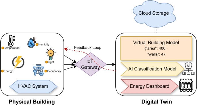
Without standardised benchmarks or empirical baseline data for categorising energy efficiency in the simulation-based dataset, the Energy Feature (EF) median value was used as a statistically neutral threshold for binary classification. This approach ensures a balanced class distribution, which is particularly important for training supervised machine learning models. While this method may not accurately reflect domain-specific thresholds, it provides a practical solution for enabling model training and performance comparison across classification algorithms. The study acknowledges this limitation and suggests that future work could involve mapping these classifications to real-world energy efficiency standards or incorporating empirical thresholds from building energy codes or green certifications. This study focuses on applying machine learning models to classify buildings based on their energy efficiency. The features selected for this classification, such as building shape, surface area, roof area, and glazing distribution, are essential factors that influence the thermal performance of buildings. These features were specifically chosen because they are known to significantly impact the building’s energy consumption patterns, and thus are highly relevant to energy efficiency analysis. The study’s results have a direct impact on building energy management, including the classification of buildings into low-energy and high-energy categories. The binary classification approach, using median values for categorization, enables us to make data-driven decisions about energy efficiency and helps simulate energy optimization in a practical, real-world context. Furthermore, the study’s use of machine learning algorithms aligns with current trends in the building energy sector, where predictive modelling is increasingly employed to make real-time energy consumption assessments and drive energy-saving strategies. Future work will explore real-time data collection through IoT sensors to better connect the methodology to building energy domain objectives, integrating live building data into the DT framework. This will allow the models to be tested in dynamic environments, with real-time performance feedback, providing more relevant insights into energy optimisation practices.